---

Table of contents

1. Chapter 2 : Training Simple Machine Learning Algorithms for Classification
   1. weight update
2. Chapter 3 : A Tour of Machine Learning Classifiers Using scikit-learn
   1. 概率，发生比(odds), 净输入(net_input) 和logit 公式之间的联系
   2. 通过activation function 更新updates
   3. overfitting and underfitting
   4. logic regression VS svm
   5. kernel SVM
   6. regularization
   7. Decision Tree
      1. information gain in Decision Tree
      2. 建立Decision Tree
      3. Random Forest
      4. K-nearest neighbors – a lazy learning algorithm
3. chapter 4 : Building Good Training Datasets – Data Preprocessing
   1. df.isna().sum()
   2. df.values
   3. 方法一：直接删除 df.dorpna(axis=?)
   4. 方法二：插值法 Imputing missing values
   5. Handle categorical missing values
      1. ordinal and nominal features
      2. ordinal features 转化
      3. convert class label into intergers
      4. one-hot encoding on nominal features
   6. 分割数据
   7. Bringing features onto the same scale
   8. Selecting meaningful features
      1. L1 and L2 regularization as penalties against model complexity
      2. 为什么L2可以减轻overfiting ， L1 可以产生sparse features
      3. Sequential feature selection algorithms
      4. Assessing feature importance with random forests
4. Chapter 5 : Compressing Data via Dimensionality Reduction
   1. Principal component analysis (PCA)
      1. sklearn 自带PCA方法
   2. linear discriminant analysis(LDA)
      1. PCA 与 LDA的区别
      2. LDA的分析流程
      3. LDA via scikit-learn
   3. kernel principal component analysis(KPCA) for nonlinear mappings
5. Chapter 6:Learning Best Practices for Model Evaluation and Hyperparameter Tuning
   1. piplines
   2. Using k-fold cross-validation to assess model performance
   3. K-fold cross-validation
   4. Debugging algorithms with learning and validation curves
      1. Addressing over- and underfitting with validation curves
      2. Fine-tuning machine learning models via grid search
   5. nested cross-validation
   6. Looking at different performance evaluation metrics
      1. precision and recall of a classification model
      2. Receiver operating characteristic (ROC)
   7. Scoring metrics for multiclass classification
   8. Dealing with class imbalance
6. Combining Different Models for Ensemble Learning
   1. Majority vote
   2. 为社么ensemble method 会比单个classifier的结果好
   3. Majority vote classifier
   4. Bagging
   5. boosting

---

Chapter 2 : Training Simple Machine Learning Algorithms for Classification

在这一章中介绍了机器学习中的神经元的发展历史。在下图中我们可以看到两种神经元。

第一种是模拟人类神经元细胞的激活机制最早提出来的。输入端模拟了树突，然后整合所有的信号，与streshold 进行比较，来判定class label(1 or -1)。

第二种改进的地方是在net input之后增加了一个activation function。这样两种神经元在对weights 进行update时，updates 的来源是不同的。第一种直接来源于output，第二种来源于activation function。前者是一个整数，后者是一个float number。这样后者可以判定偏移正常class label 的程度。而第一种不可以。

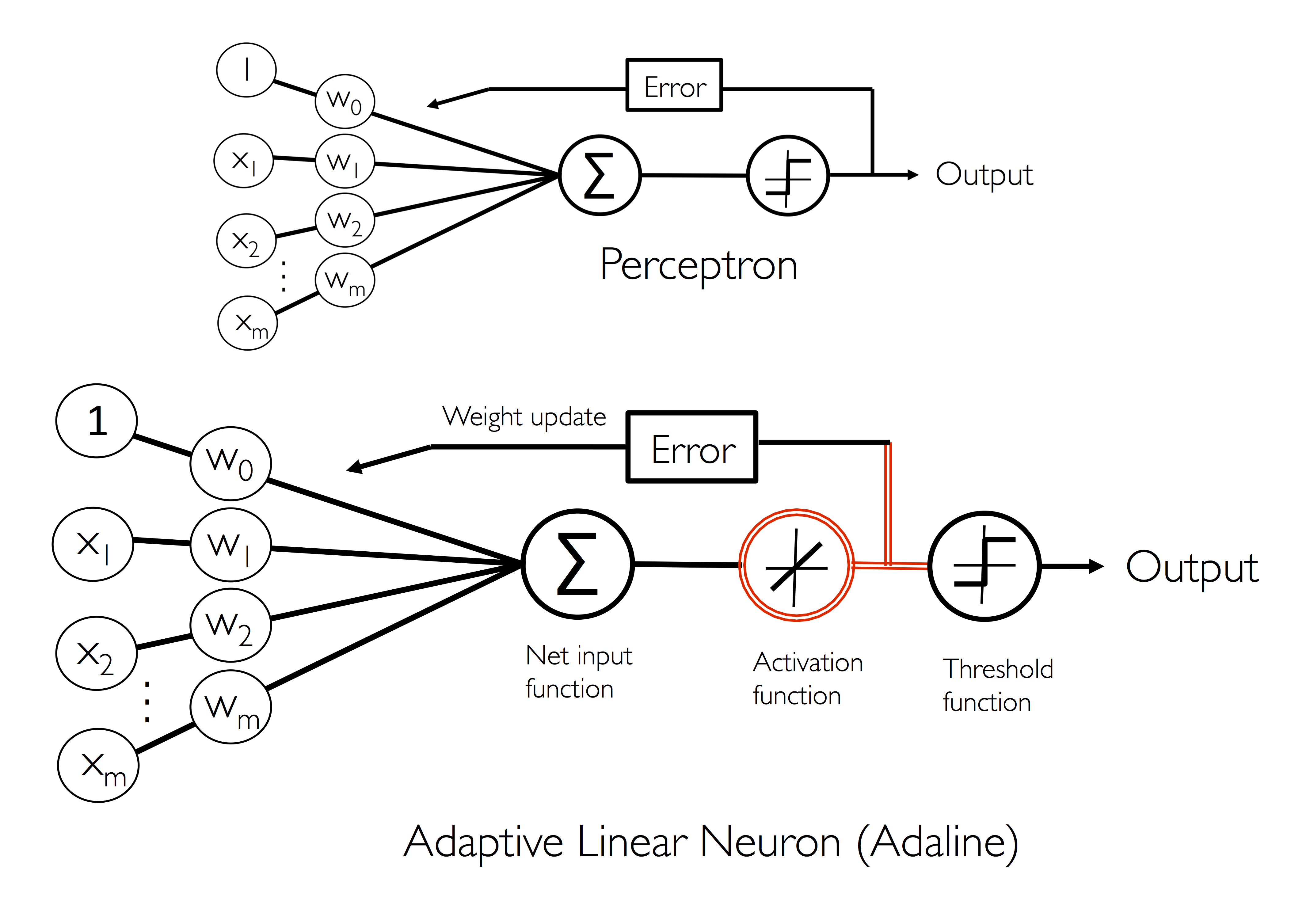
同时这一章还介绍了为什么会有bias，在perceptron中为了使threshold=0.我们认为添加了一个bias，并且bias存放在weights数列的第一个。

weights在初始化时，其应该是很小的数，但不能为0，如果为0则书本上说其weights的变化只是scaler的变化，而没有方向上的变化。同时使用w = np.random.norm(loc=0.0, scale=0.1, size = 1+ x.shape[1])来初始化weights。

在写code时应培养良好的document。在本章中可以借鉴一下：

“”“function or class definition,具体是干什么的

Parameters
------
p1 : type
    definition
p2 : type
    definition
    
Returns
-------
r1 : type
    definition
r2 : type

Examples
-------
give some simple examples

Other
-------
Description

“”“

weight update

w += det_w

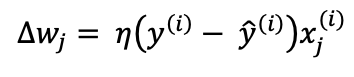
以上是第一种神经元Perceptron的weights进行update时，weights变化

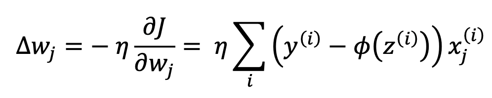
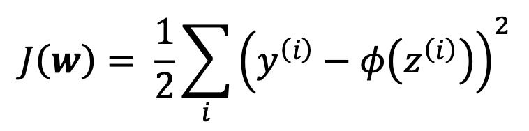
以上是第二种神经元ada的weights 进行update时weights的变化量。其来源于以下cost 函数。只需要对wj进行求偏导就可以得到以上公式。

两者的区别如下：

1. perceptron ： 每一个example(row)对weight进行更新一次； ada：公式里面有求和符号，因此是对所有的example遍历完之后再更新weights。后者叫做Batch Gradient descent。
2. 对于perceptron，error = yi - y^i 其中output是class label，即 1 or -1。而ada error 中的output 是一个float number。
3. perceptron：deta_w 中的x是一个row中的fetures。ada：是一个点积。

如果我们的数据量很大，那么遍历完所有的examples再更新weights则不实际。因此我们也可以每一个example 更新一次weights，这叫做stochastic gradient descent。

对于learning rate(eta)超参数。如果太大，则会发生overshoot，即在minumn点来回的走动。如果太小，则聚合太慢。

对于data中数据数量级不一致的情况，例如有的列为0.09，有的列为19800，那么显然直接使用两者的数据进行parameter fiting。后者影响会很大，而前者影响小。也会影响聚合速度。因此我们需要对数据进行normalize。常见的normalize为 (data - mean)/std使用numpy 很简单：(x-x.mean())/x.std()

为什么要添加activation：这是因为activation得出的结果与true label的error可以衡量与ture label 的距离相差多少。而使用threshold后的结果，则不能凸显与之程度。在这一章中使用的是linear activation，即直接输出，没有变化。

神经元的数据流动过程

1. net input ：net_input = np.dot(X,self.w_[1:]) + self.w_[0]. self.w_[0] is the bias
2. activation function
3. compute the error : error = true_labe - output. here output came from activation. But if the perceptron nueron, then it is the final predicted label
4. get the predicted label by comparing the threshold
5. do the next example or next batch

Chapter 3 : A Tour of Machine Learning Classifiers Using scikit-learn

The five main steps that are involved in training a supervised machine learning algorithm can be summarized as follows:

1. Selecting features and collecting labeled training examples.
2. Choosing a performance metric.
3. Choosing a classifier and optimization algorithm.
4. Evaluating the performance of the model.
5. Tuning the algorithm.

在这一章中介绍了sklearn 中几个常用的分类算法：logic regression，svm，decision tree, random forest, KNN(k nearest neighbours)。

解决的疑惑有：

1. logic regresssion ：sigmoid activation function的由来。
2. 各算法的优缺点。后面详细说明
3. decision tree 判定node的计算过程：通过IG(information gain)来决定对哪个feature 进行分割
4. random forest 是在整个dataset 中随机有放回的选择一些examples，然后再随机选择一些features来build decision tree。而 sklearn中默认情况下是直接使用全部的dataset，然后随机选择subfeature来进行build tree组成random forest。
5. overfitting and underfitting
6. regularization

概率，发生比(odds), 净输入(net_input) 和logit 公式之间的联系

首先明确几个感念，具体细节可参考csdn：

• 概率：概率是指一个事件发生的可能性
• 发生比:发生比指一件事发生与其不发生的概率之比，
• Logit :Logit是给发生比取对数，即log(Odds)，其中log是自然对数。
• net_input = X*w

因为我们从上一章中了解到了神经元中的信息流动过程。知道了net_input。在得到net_input之前的过程基本都是一致的。那么在perceptron中直接使用net_input 经过threshold的结果（label）作为error 的参数 ·error = true_labe - label；而在Ada 中则是使用linear activation function。即直接使用net_input来计算error:error = true_label - net_input。

由于最后一种神经元采取的是概率作为评判结果。因此对于二分类模型来说，结果在[0,1]之间。因此我们要使net_input经过activation function 之后结果也在[0,1]之间。

那么为什么会引入发生比和logit呢？我想到的是这两者与概率有关。第一位吃螃蟹的人尝试了以下方法，觉得不错。记住我们的目的是要求概率，且与net_input扯上关系。

• 可以让 p = net_input 吗？

不可以，因为这样的话net_input的范围只能控制在[0,1]，不方便update weights。太窄了。

• 可以让odds = net_input 吗？

不可以，因为发生比有不对称性, 当概率从0.1增加到0.2，时，发生比增加了0.139；当概率从0.8增加到0.9时，发生比却增加了5，虽然概率的增量相同，但发生比的增量却大大的不同。其他例子可以参考csdn

• 可以让logit = net_input 吗？

为了解决odds的不对称性，引入了logit。因为log函数容易计算和求导。因此让logit(p) = z, here z = net_input = X*w.

log(p/1-p) = z

• p/(1-p) = e^z
• p = e^z/(1+e^z)
• p = 1/(1+e^-z)

到这里我们把概率和net_input联系在了一起，并且1/(1+e^-z)就是activation function。

通过activation function 更新updates

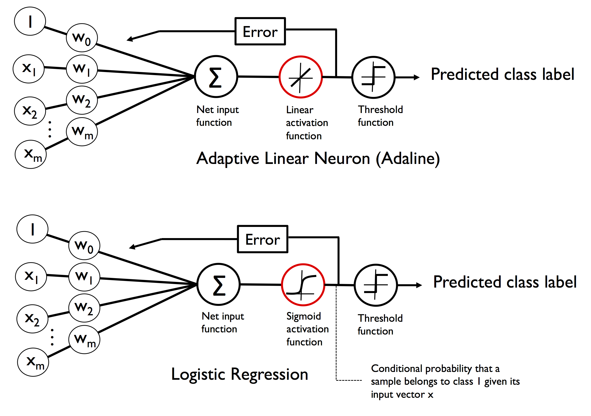
从图中可以看出 ada 与 logic regression 之间的不同之处：

1. activation function是不同的。ada 是linear activation；logic regresion是sigmoid activation。
2. logic regression 可以求得当前class label 的概率。

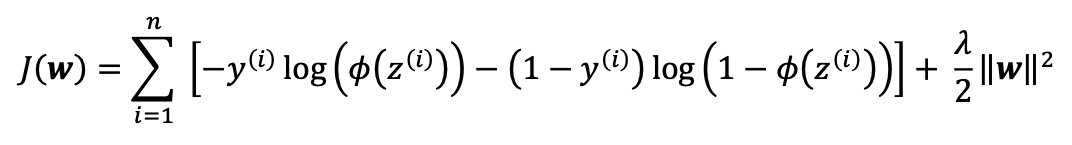
logic regression 的cost function是求得最大的likelihood. 求deta_w的过程如下：

1. 获得最大likelihood，这是一个乘积公式
2. 求log转化为求和公式

为什么转化为求和公式：

1. 因为乘积会导致数据溢出。
2. 求导方便

overfitting and underfitting

If a model suffers from overfitting, we also say that the model has a high variance,

Similarly, our model can also suffer from underfitting (high bias), which means that our model is not complex enough to capture the pattern in the training data well and therefore also suffers from low performance on unseen data.

overfitting : high variance underfitting : high bias

logic regression VS svm

logic regression 更容易受到outlier data 的影响。而svm 可以通过调节C值 来改变svm的regularization的程度。

kernel SVM

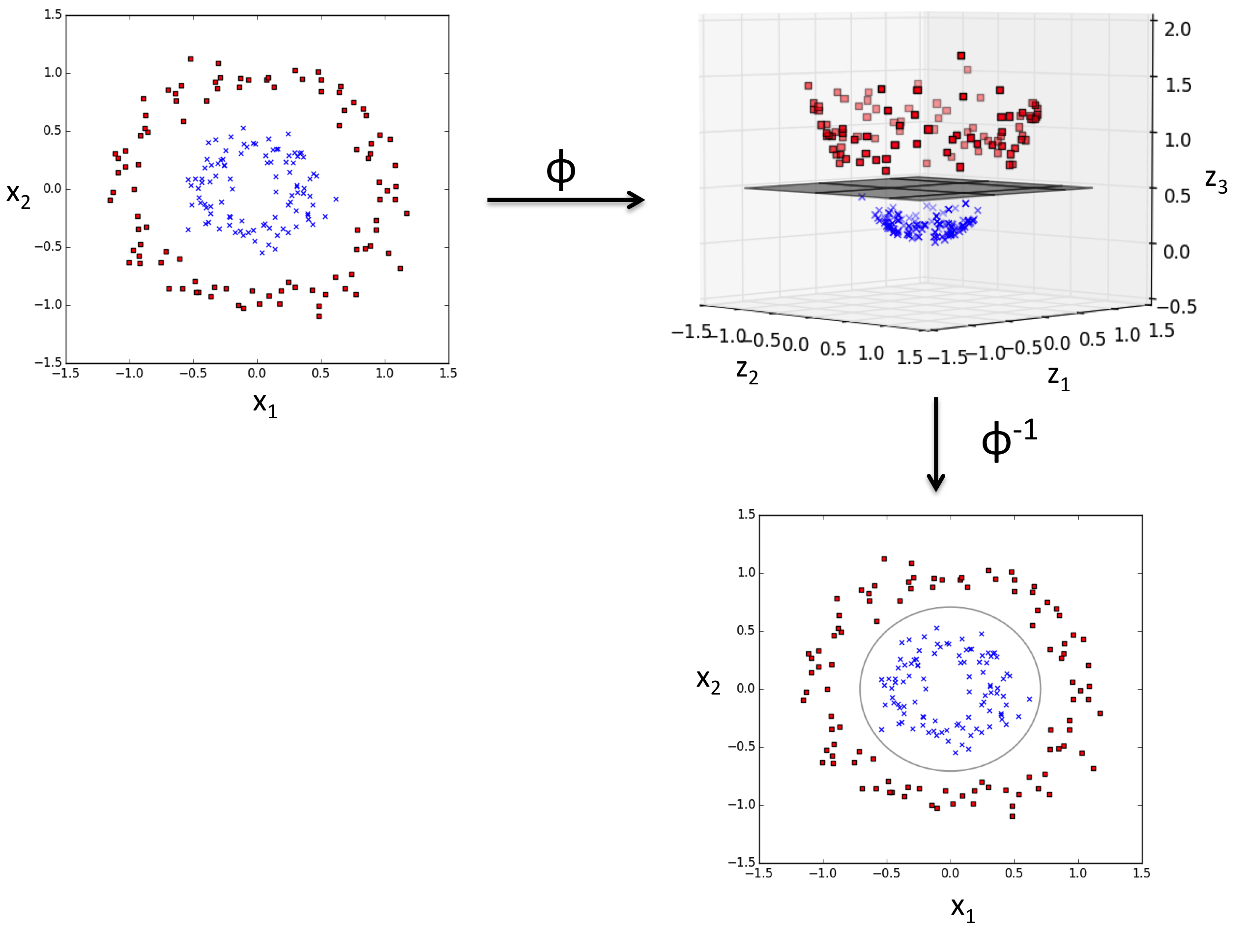
如果data 是可以进行线性划分的，那么使用linear SVM就可以了。如果不是线性划分的(nonlinear sepratable),那么可以使用kernel SVM进行分割。其基本思路是把在当前维度上不可分的数据进行升维。在高维上就可以转化成为线性可分了。如下图所示：

regularization

The concept behind regularization is to introduce additional information (bias) to penalize extreme parameter (weight) values.

The most common form of regularization is so-called L2 regularization (sometimes also called L2 shrinkage or weight decay), which can be written as follows:

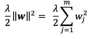
1. 之所以叫做weight decay 是因为偏移量与weight 有关。
2. 同时为了做regularization也要进行feature normalization，这样各weights之间有可比较性。

Decision Tree

• 如何分割每个node

以下公式是decision tree 的目标函数。即每次分割都会使IG(D,f)最大。

Here, f is the feature to perform the split; 𝐷𝑝 and 𝐷𝑗 are the dataset of the parent and jth child node; I is our impurity measure; 𝑁𝑝 is the total number of training examples at the parent node; and Nj is the number of example in the jth child node.

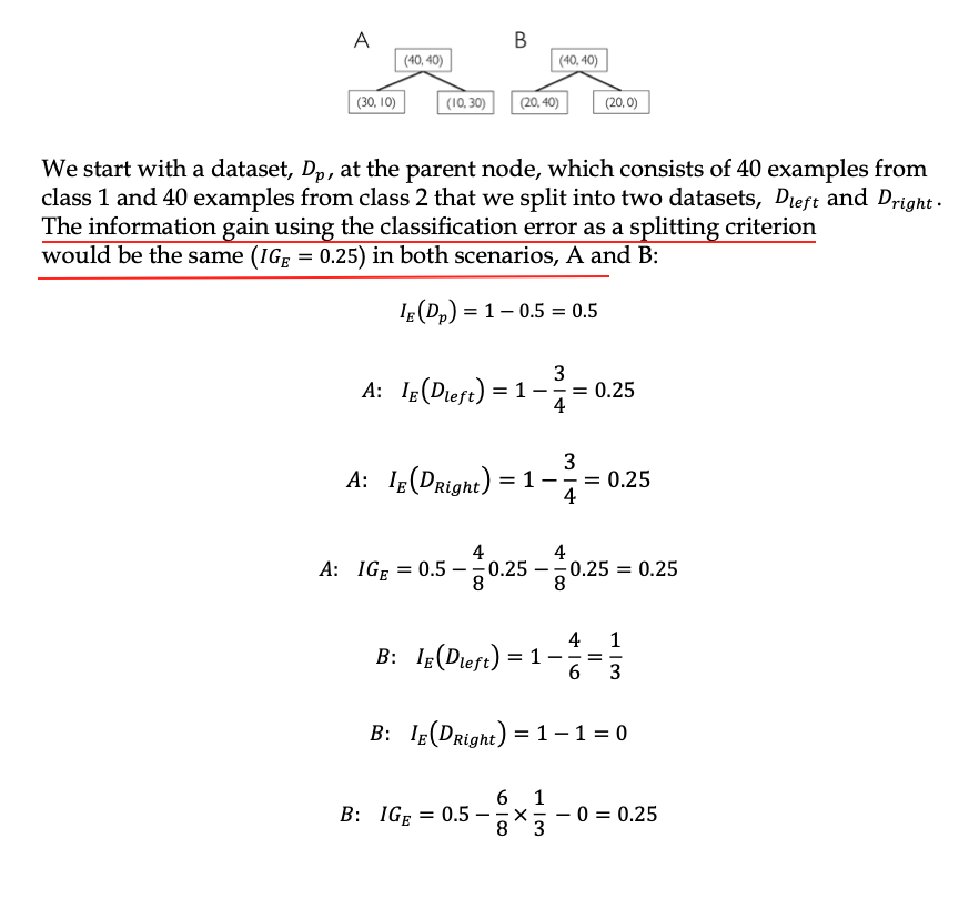
The information gain is simply the difference between the impurity of the parent node and the sum of the child node impurities—the lower the impurities of the child nodes, the larger the information gain.

为了简单，一般使用binary decision tree。因此以上公式简化为如下公式。只有左右两个child。

information gain in Decision Tree

在以上公式中的I(D)即不纯净度检测(impurity measure)可以有以下三种方法：

1. Gini impurity
2. Entropy
3. Classification error

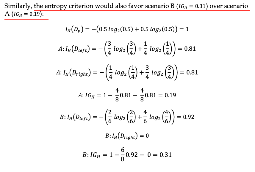
• Entropy equation

前提是non-empty class p(i|t) != 0 Therefore, we can say that the entropy criterion attempts to maximize the mutual information in the tree.

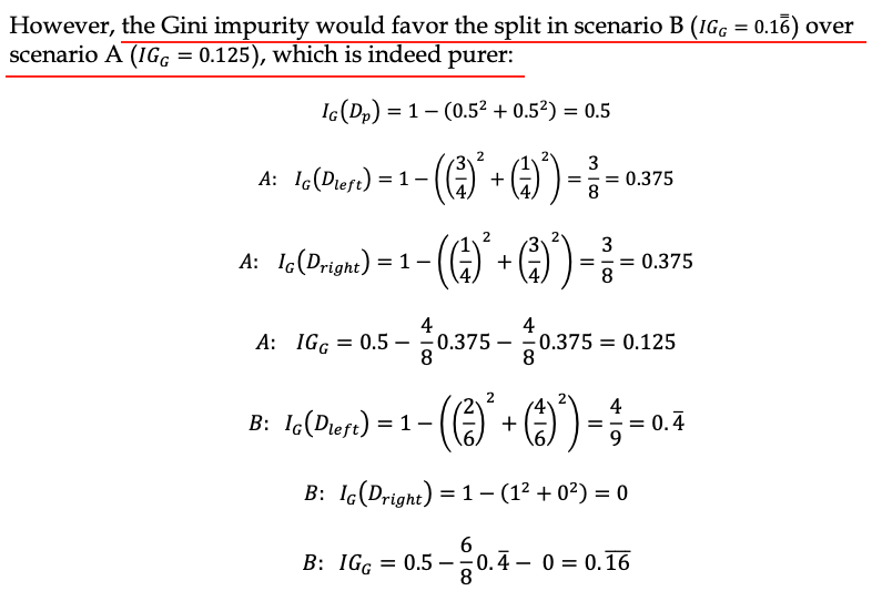
• Gini impurity

The Gini impurity can be understood as a criterion to minimize the probability of misclassification:

Gini 可以认为是尽量使误分类的class概率最小。Gini 与Entropy 在perfectly mixed 的情况下，值最大。如果两个class，每个class 的概率为0.5，那么Gini的值是1-2*0.5^2=0.5; entropy 的结果是1. 使用Gini 和 Entropy 的结果都差不多。

• classification error

classification error 可以用于剪枝，但是并不适合用于树的增长。因为它对每个nodes中class概率的变化并不敏感。虽然probability有变化，但是很可能结果一致。但是Gini和Entropy却可以查出这些变化，并给出合理的结果。

从下面的案例中我们可以看出三者的不同之处：

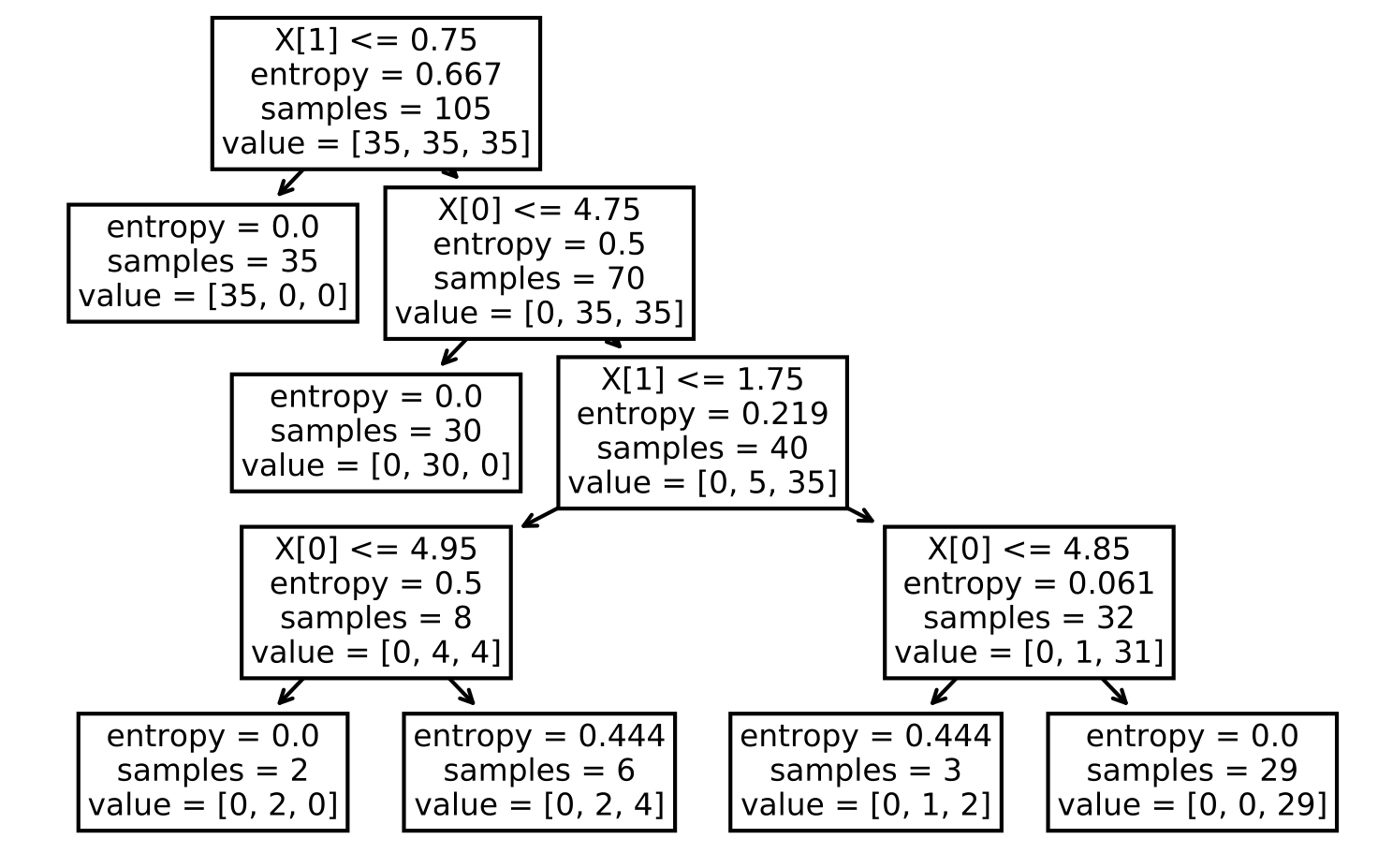
建立Decision Tree

from sklearn.tree import DecisionTreeClassifier
tree_model = DecisionTreeClassifier(criterion='gini',
                                   max_depth=4,
                                   random_state=1)
tree_model.fit(X_train,y_train)

from sklearn import tree
tree.plot_tree(tree_model)
plt.show()

通过使用 tree.plot_tree来显示tree 的内部每个node是如何划分的。

Random Forest

The random forest algorithm can be summarized in four simple steps:

1. Draw a random bootstrap sample of size n (randomly choose n examples from the training dataset with replacement).
2. Grow a decision tree from the bootstrap sample. At each node: a. Randomly select d features without replacement. b. Split the node using the feature that provides the best split according to the objective function, for instance, maximizing the information gain.
3. Repeat the steps 1-2 k times.
4. Aggregate the prediction by each tree to assign the class label by majority vote.

In the step 2, instead of evaluating all features to determine the best split at each node, we only consider a random subset of those.

• Advantage of Random Forest

1. we don’t have to worry so much about choosing good hyperparameter values. We typically don’t need to prune the random forest since the ensemble model is quite robust to noise from the individual decision trees.
2. The only parameter that we really need to care about in practice is the number of trees, k, (step 3) that we choose for the random forest.
3. Other parameters inclue the size, n, of the bootstrap sample (step 1), and the number of features, d, that are randomly chosen for each split (step 2.a), respectively.

K-nearest neighbors – a lazy learning algorithm

KNN is a lazy learning algorithm and don’t have parameters.

KNN 并不适用于维度很高的数据。因为在高维度上KNN的结果会变得很疏松。因此如果是高维度的数据，应该首先进行降维。

chapter 4 : Building Good Training Datasets – Data Preprocessing

df.isna().sum()

使用df.isna().sum()查看每个column中有多少missing values。

df.values

使用df.values将dataframe转化为numpy。sklearn 中主要是对numpy的数据进行处理。现在sklearn中很多function都可以支持pandas。所以如果可以转化为numpy则尽量转化为numpy后再使用sklearn。

方法一：直接删除 df.dorpna(axis=?)

最简单粗暴的方法就是使用df.dropna直接删除。

• 如果想删除带有NaN的rows： df.dropna(axis=0)
• 删除带有NaN的columns ： df.dropna(axis=1)
• only drop rows where all columns are NaN : df.dropna(how='all')
• drop rows that have fewer than 4 real values : df.dropna(thresh=4)
• only drop rows where NaN appear in specific columns (here: ‘C’): df.dropna(subset=['C'])

方法二：插值法 Imputing missing values

由于直接删除数据有以下缺点：

• 如果删除太多的数据导致数量太少，难于分析挖掘出有用的数据。
• 如果删除了column，而此column可能与对class进行分离很重要，导致分类不准确。

鉴于此，更常用的方法是使用插值法。常用的差值方法是使用均值(mean imputation)。

• 使用sklearn 中的SimpleImputer很方便完成。

from sklearn.impute import SimpleImputer
import numpy as np
imr = SimpleImputer(missing_values=np.nan, strategy='mean')
imr = imr.fit(df.values)
imputed_data = imr.transform(df.values)
imputed_data

SimpleImputer 对numpy数据进行处理。因此使用df.values把dataframe转化为numpy. strategy参数除了mean之外，还有median or most_frequent。当数据是categorical feature 时使用most_frequent是非常有帮助的。

• 使用df.fillna(df.mean()) 填补缺失值

使用df.fillna(df.mean())来填补缺失值(均值)

Handle categorical missing values

以下python代码的案例如下

df = pd.DataFrame([
          ['green', 'M', 10.1, 'class2'],
           ['red', 'L', 13.5, 'class1'],
         ['blue', 'XL', 15.3, 'class2']])
df.columns = ['color','size','price','classlabel']

ordinal and nominal features

• ordinal features : Ordinal features can be understood as categorical values that can be sorted or ordered. 例如衬衫的size 大小， XL > L > M.

• nominal features don’t imply any order ： 衬衫的颜色是nominal feature，我们不能说red > green。

ordinal features 转化

我们可以认为设定ordinal features mapping把data 中的categorical featu 转化为integer value。

size_mapping = {
    'XL':3,
    'L':2,
    'M':1
}
df['size'] = df['size'].map(size_mapping)

以上的mapping我们认为XL=L+1=M+2而得出来的。如果我们不知道这种relationship，但是我们知道XL>L>M。我们可以用另一种形式的encoding。我们把>M or >L的size转化为binary value。

df['x>M'] = df['size'].apply(lambda x:1 if x in {'L','XL'} else 0 )
df['x>L'] = df['size'].apply(lambda x:1 if x == 'XL' else 0)

convert class label into intergers

因为sklearn对数字处理很在行，对于categorical values并不友好。因此我们最好把class label转化为interger方便machine learning model进行处理。

• 使用mapping

class_mapping = {k:i for i,k in enumerate(np.unique(df['classlabel'].values))}

df['classlabel'].map(class_mapping)

• 使用sklearn自带的LabelEncoder

from sklearn.preprocessing import LabelEncoder
class_le = LabelEncoder()
y = class_le.fit_transform(df['classlabel'].values) # 转化为integer
class_le.inverse_transform(y) # 转化为categorical values

one-hot encoding on nominal features

对于nominal features，我们不能使用mapping 或者LabelEncoder转化成为interger。因为这样的话，machine learning model 会认为各integer之间存在大小关系。因此我们需要把每个nominal value转化为一个dummy feature(binary value)。即这个value是否是存在的。

• 方法一：使用sklearn自带的 OneHotEncoder

from sklearn.preprocessing import OneHotEncoder
X = df.values

color_ohe = OneHotEncoder()

color_ohe.fit_transform(X[:,0].reshape(-1,1)).toarray()

因为sklearn中的function 对numpy数据进行处理，因此第一步便是把dataframe的数据转化为numpy数据(df.values)。X[:,0].reshape(-1,1) 这一步操作是把X中的某一列提取出来(此时是row的形式)，然后再转化为nX1的matrix形式，因为sklearn中的function 中的fit_transform只对matrix进行处理。为了显示结果使用toarray()

• 方法二：使用sklearn自带的 ColumnTransformer

from sklearn.compose import ColumnTransformer

c_transf = ColumnTransformer([
    ('onehot',OneHotEncoder(),[0]),
    ('nothing','passthrough',[1,2])
])

c_transf.fit_transform(X).astype(float)

The ColumnTransformer accepts a list of (name, transformer, column(s)) as above. 最后我们使用astype把numpy的数据进行格式转换，将object格式转化成为float格式。

• 使用DataFrame自带的get_dummiesmethod

pd.get_dummies(df[['price', 'color', 'size']])

在上面的转化中我们对每一个nominal vlaue都进行了dummy binary value转化。这样导致我们转化后的结果是高度相关的。例如当color_blue=0 and color_green=0，那么color_red一定是1.这样高度相关的matrix会导致matrix在计算时非常困难(inverse)。因此我们要在dummy values中删除一列。

pd.get_dummies(df[['price','color','size']],drop_first=True)

color_ohe = OneHotEncoder(categories='auto', drop='first')
c_transf = ColumnTransformer([
    ('onehot',color_ohe,[0]),
    ('nothing','passthrough',[1,2])
])
c_transf.fit_transform(X).astype(float)

在pd.get_dummies中添加参数drop_first=True;在OneHotEncoder中添加参数categories='auto', drop='first'

分割数据

使用sklearn自带的train_test_split对数据进行分割

from sklearn.model_selection import train_test_split

X_train,X_test,y_train,y_test = train_test_split(X,y,test_size=0.3,stratify=y)

分割的比例为train:test = 7:3;Providing the class label array y as an argument to stratify ensures that both training and test datasets have the same class proportions as the original dataset.

Bringing features onto the same scale

feature scaling 是非常重要的一步。除了 Decision trees and random forests 这两个algorithm不需要进行feature scaling之外，绝大部分machine learning algorithm需要feature scaling。例如 gradient descent optimization algorithm

feature scaling 的重要性: 如果两个column feature 的scale不同。一个是1到10，另一个是1 到1000.那么在training 的过程中，the algorithm会忙于对scale大的那个feature的weights 进行update。

feature scaling 的两种形式：

• normalization:

即 min-max scaling的另一种形式。可以把数据限制在[0,1]之内。因此当我们需要把数据限制在某一范围内时，min-max scale是非常有用的。

Here, x^i is a particular example, x_min is the smallest value in the feature column, and x_max is the larget value

sklearn 中的MinMaxScaler对数据进行min-max scaling

from sklearn.preprocessing import MinMaxScaler

mms = MinMaxScaler()
X_train_norm = mms.fit_transform(X_train)
X_test_norm = mms.transform(X_test)

• standardization：

u_x is the sample mean of a particular feature colum, and \sigma_x is the correspongding standard deviation.

standardization 主要是用于machine learning algorithms，尤其是在optimization 算法中，例如 gradient descent.

• 这是因为我们在weights初始化时往往把weights初始化为非常接近于0的随机数。这时我们使用standardization 把feature也设置成与weights parameter同样的standard normal distribution(zero means and unit variance)，这样weights会学习的更快
• 另一个原因是standarization 保留outliers 的有用信息，相较于min-max scaling，standarization对outliers不敏感。

我们可以使用sklearn中的StandardScaler method对features 进行standardization。

from sklearn.preprocessing import StandardScaler

stdsc = StandardScaler()
X_train_std = stdsc.fit_transform(X_train)
X_test_std = stdsc.transform(X_test)

• RobustScaler

如果dataset比较小，且有很多outliers，又或者发生overfitting，那么RobustScaler是一个不错的选择。

Selecting meaningful features

当我们在训练模型时发生overfitting，原因是当前的模型对与当前的dataset来说太复杂了，导致模型有很高的variance and has a high generalization error.

Common solutions to reduce the generalization error are as follows(阻止overfitting的方法):

• Collect more training data
• Introduce a penalty for complexity via regularization
• Choose a simpler model with fewer parameters
• Reduce the dimensionality of the data

第一条，收集更多的数据并不实用。

1. 我们不知道是否是由于收集的feature nosie 太多导致模型发生high variance，因此收集更多的samples也没有用。
2. 成本太高，或者根本没有办法收集更多的samples。

下面我们看一下通过regularization和dimensionality reduction via feature selection。前一种对于有weights 需要调节的model来说很有用，而第二种，对于没有weights要调节的模型（Decsion tree and Random Forest）来说有用。

L1 and L2 regularization as penalties against model complexity

• L2 regularization:

• L1 regularization:

In contrast to L2 regularization, L1 regularization usually yields sparse feature vectors and most feature weights will be zero.

当我们的数据有很多不相关的feature时(这里的不相关是指与model要预测的结果不相关，应该不是指feature之间的相关性)，或者feature的数目已经大于sample的数目时，L1 regularization 可以用于feature selection。

为什么L2可以减轻overfiting ， L1 可以产生sparse features

下面用几何方法进行表示，可以清晰地看出两者之间的区别以及两者是如何作用于weights用于减轻overfitting。

A geometric interpretation of L2 regularization

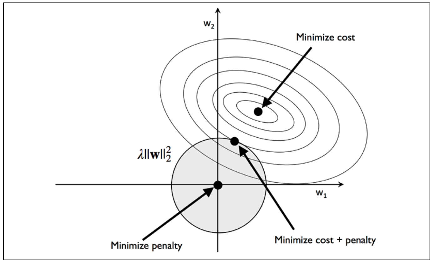
由于L2的图形在坐标系中是一个圆，而cost function这里使用的是sum of squared errors(SSE)。虽然其他的cost function与之不同，但是基本思路是一致的。

我们的目的是到达cost function中间的Minimize cost，L2的作用则是把weights限定在这个shaded圈中。那么距离Minimize cost最近的圈中的点则是相交的边界点。我们这里的regularization的值可以认为是一个定值，即L2的表达值是一个定值。如果lambda变大，那么w就会变小，这个shaded 圈也会变小，而weights的变化范围也会变小。如果lambda趋于无穷大，则w会趋于零。

To summarize the main message of the example, our goal is to minimize the sum of the unpenalized cost plus the penalty term, which can be understood as adding bias and preferring a simpler model to reduce the variance in the absence of sufficient training data to fit the model.由于weights的变化范围变窄了(the intersection of shaded ball and cost function)，因此可以认为model变简单了。

A geometric interpretation of L1 regularization

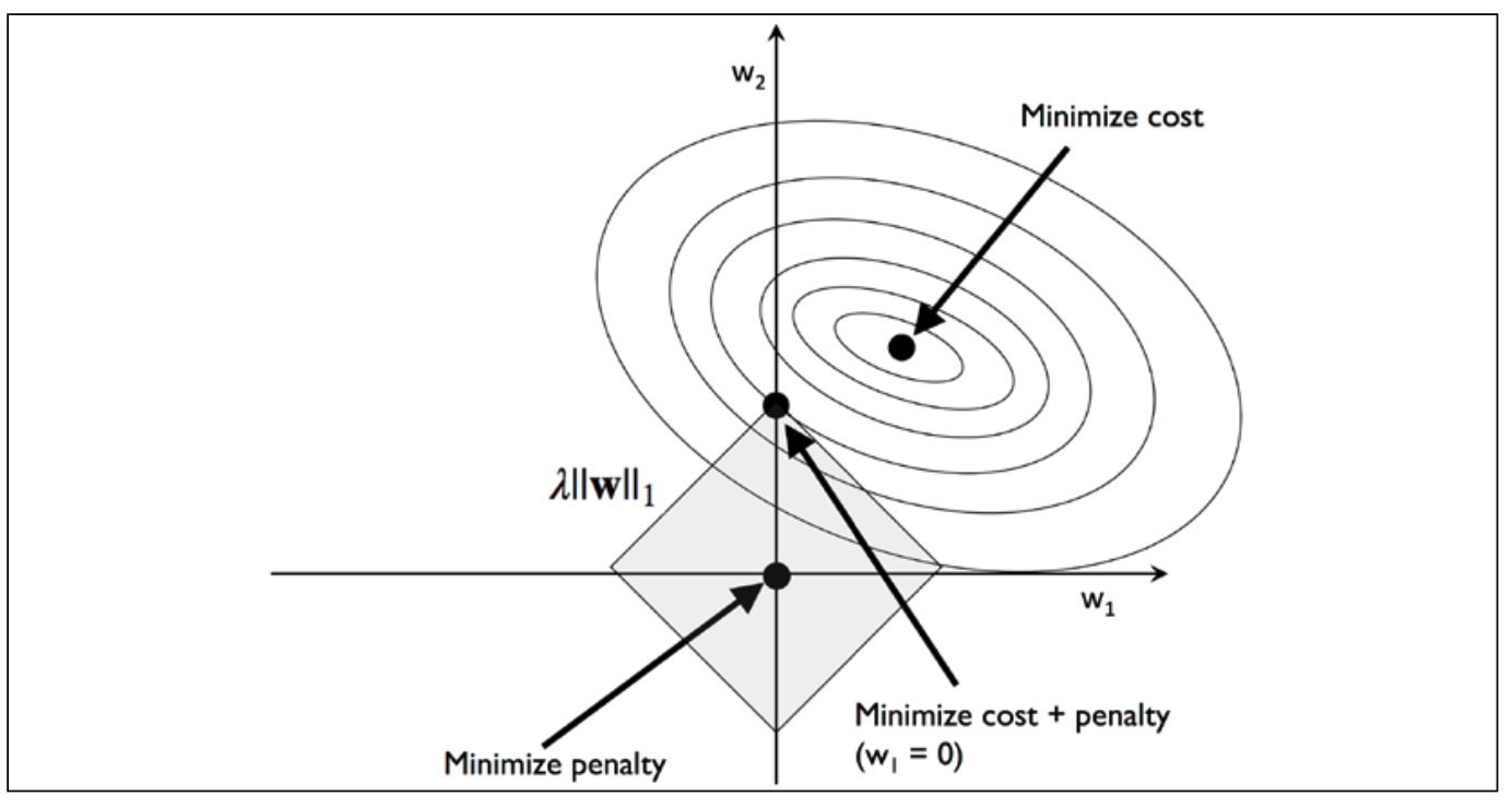
L1 的表达式是绝对值，因此它的图形是一个矩形，中心是原点。其与cost function的交界处存在与轴上，例如在图中w1=0。如果是多维的数据，那么交界在其中一维上，那么其他维则为0，就会导致sparse features。我们可以通过这个特征提取重要的feature。这里认为不等于0的feature是重要的feature。

下面使用sklearn来查看L1的效果：

from sklearn.linear_model import LogisticRegression

lr = LogisticRegression(penalty='l1',
                        C=1.0, # C值是lambda的倒数，C值越小labmda越大，更多的feature会变为0，feature越稀疏。
                        solver='liblinear',
                        multi_class='ovr'
                       )

lr.fit(X_train_std,y_train)

lr.score(X_train_std,y_train)

lr.score(X_test_std,y_test)

lr.intercept_ 

lr.coef_ # weights 的值

• lr.intercept_ : 由于使用的one vs rest(OvR) 方法，因此会有三个截距即bias，the first intercept belongs to the model that fits class 1 versus classes 2 and 3, the second value is the intercept of the model that fits class 2 versus classes 1 and 3, and the third value is the intercept of the model that fits class 3 versus classes 1 and 2

• In scikit-learn, the intercept_ corresponds to 𝑤0(bias) and coef_ corresponds to the values 𝑤j(weights) for j > 0.

Sequential feature selection algorithms

L1适用于有weights可以调节的模型。如果没有weights可以进行调节模型，那么我们就需要 dimensionality reduction。

减少维度有两种方法：

• feature selection ：we select a subset of the original features。从原有的features中选择出比较重要的feature。
• feature extraction ： derive information from the feature set to construct a new feature subspace。从原有的features space构建新的features subspace，即通过转化成新的features，并不是简单的提取。

Sequential feature selection(SBS)属于第一种，这是一个greedy algorithm。 At each stage we eliminate the feature that causes the least performance loss after removal.

Assessing feature importance with random forests

使用sklearn 自带的random forest来评估feature的重要性。

from sklearn.ensemble import RandomForestClassifier

feat_labels = df_wine.columns[1:]
forest = RandomForestClassifier(n_estimators=500,
                                random_state=1
                               )
forest.fit(X_train,y_train)

importances = forest.feature_importances_

indices = np.argsort(importances)[::-1]

for f in range(X_train.shape[1]):
    print("%2d) %-30s %f"% (f+1,
                           feat_labels[indices[f]],
                           importances[indices[f]]))

plt.title('Feature Importance')
plt.bar(range(X_train.shape[1]),
        importances[indices],
        align='center'
       )
plt.xticks(range(X_train.shape[1]),
           feat_labels[indices], rotation=90
          )
plt.xlim([-1, X_train.shape[1]])
plt.tight_layout()
plt.show()

图可参考python知识点

从上面我们可以根据importance得出features的重要性。我们也可以通过sklearn自带的SelectFromModel来选择features。

from sklearn.feature_selection import SelectFromModel
sfm = SelectFromModel(estimator=forest, threshold=0.1, prefit=True) 
X_selected = sfm.transform(X_train)

forest 是已经训练好的模型，因为prefit=True。 threshold=0.1,是feature importance的limit，The estimator should have a feature_importances_ or coef_ attribute after fitting.

Chapter 5 : Compressing Data via Dimensionality Reduction

通过减少数据的维度来浓缩数据对于数据的储存和分析非常重要。

• 因为对于没有weights进行调节的model，我们可以通过减少维度来提升model的performance。
• reducing the curse of dimensionality

The difference between feature selection and feature extraction is that while we maintain the original features when we use feature selection algorithms, such as sequential backward selection, we use feature extraction to transform or project the data onto a new feature space.

In the context of dimensionality reduction, feature extraction can be understood as an approach to data compression with the goal of maintaining most of the relevant information. 在减少维度的同时尽可能保留相关的信息。

这一章涵盖以下topics about Dimensionality Reduction:

• Principal component analysis (PCA) for unsupervised data compression
• Linear discriminant analysis (LDA) as a supervised dimensionality reduction technique for maximizing class separability
• Nonlinear dimensionality reduction via kernel principal component analysis (KPCA)

Principal component analysis (PCA)

PCA的目的是在原始数据空间中找到互相垂直的维度，在一维度下，数据之间的差异最大(variance), 我们认为variance包含了数据的信息，差异越大包含的信息越多。此时的维度与原始数据的维度不同，此时的维度属于原始数据空间的subspace，其维度数 <= 原始维度数。

那么如何才能找到subspace中的维度呢？get the eigen pairs( eigenvectors,eigen values) from feature matrix ，通过eigenvalues的大小把eigen vectors 组成一个matrix M，然后通过xM=x_prime,求得新的x。

因为各个维度之间的数据要进行比较，要有可比性，因此在求eigen pairs之前，应该进行standardization。

步骤如下：

1. Standardize the d-dimensional dataset.
2. Construct the covariance matrix.
3. Decompose the covariance matrix into its eigenvectors and eigenvalues.
4. Sort the eigenvalues by decreasing order to rank the corresponding eigenvectors.
5. Select k eigenvectors, which correspond to the k largest eigenvalues, where k is the dimensionality of the new feature subspace (𝑘 ≤ 𝑑).
6. Construct a projection matrix, W, from the “top” k eigenvectors.
7. Transform the d-dimensional input dataset, X, using the projection matrix, W, to obtain the new k-dimensional feature subspace.

sklearn中有自带的function可以求得feature matrix 的PCA，具体的每一步分析书本中有涉及，写的很详细，这里不赘述。

其中几个关键点涉及一下：

1. 第一主成分含有的variance最大。即最大的eigenvalue对应的eigenvector转化后的feature。
2. covariance(相关性) between two features x_j and x_k:

\mu_j and \mu_k是相应列的均值。如果我们有13列的features，那么我们可以得到13x13 covariance matrix sigma。

1. eigenvalue and eigenvector 的关系

第一个是covariance matrix，第二个是eigen vecotr，第三个是eigenvalue。

1. 我们得到top k eigenvectors后，然后把这些vector合并成nxk的matrix W，然后再用XW转化为新的features。

sklearn 自带PCA方法

from sklearn.decomposition import PCA
pca = PCA(n_components=2) # 初始化，设定剩余的维度数
X_train_pca = pca.fit_transform(X_train_std) #转化数据X_train_std.注意这里转化的数据是standrization 后的数据
X_test_pca = pca.transform(X_test_std) # 转化X_test_std

如果参数n_components=None，则所有的principle components都会被保存，如果设定了具体的数值，如n_components=2,则只会保留2个主成分。

pca = PCA(n_components=None)
X_train_pca = pca.fit_transform(X_train_std)
pca.explained_variance_ratio_ # 各主成分的占比
pca.explained_variance_ # 各主成分的大小

linear discriminant analysis(LDA)

LDA 是Supervised data compression，因此它会用到class label的信息。

PCA 与 LDA的区别

• 两者都是线性转化( linear transformation techniques) 把高维度的数据转化成为低维度线性数据
• PCA是unsupervised；LDA是supervised。

LDA的分析流程

LDA假设分析的数据是normally distributed.但是有时不满足也可以使用这个LDA技术来进行降维。分析class labels是否是满足normally distriubted可以使用np.bicount()来查看每个label的distribution

let’s briefly summarize the main steps that are required to perform LDA:

1. Standardize the d-dimensional dataset (d is the number of features).
2. For each class,compute the d-dimensional mean vector.
3. Construct the between-class scatter matrix,S_B, and the within-class scatter matrix,S_w.
4. Compute the eigenvectors and corresponding eigenvalues of the matrix,S_w^-1S_B.
5. Sort the eigenvalues by decreasing order to rank the corresponding eigenvectors.
6. Choose the k eigenvectors that correspond to the k largest eigenvalues to construct a 𝑑 × 𝑘-dimensional transformation matrix, W; the eigenvectors are the columns of this matrix.
7. Project the examples onto the new feature subspace using the transformation matrix, W.

由以上我们可以看出从第5步开始LDA 与PCA方法相同。之所以说LDA是supervised method是因为在第2步使用到了class labels的信息。

在LDA中可以得到的最后降低的维度数为c-1, c是 class的种类数目。(In LDA, the number of linear discriminants is at most c-1, where c is the number of class labels)

LDA via scikit-learn

LDA每一步的详细过程在书本中有介绍，比较复杂，这里不再赘述。使用sklearn自带的function可以完成LDA。如下：

from sklearn.discriminant_analysis import LinearDiscriminantAnalysis as LDA
lda = LDA(n_components=2) # n_components <= Using min(n_features, n_classes - 1) = min(13, 3 - 1) = 2 components.
X_train_lda = lda.fit_transform(X_train_std,y_train) # after standarization

lr = LogisticRegression(multi_class='ovr', random_state=1,
                       solver='lbfgs')

lr.fit(X_train_lda,y_train)

• n_components 要满足min(n_features, n_classes - 1)
• lda转化要先把数据进行standarization

kernel principal component analysis(KPCA) for nonlinear mappings

PCA 与 LDA都是线性转化，要求数据必须是线性可分割的。如果数据不是线性可分割的，那么这两种方法则没有了用武之地。这时要使用kernel principal component analysis(KPCA).

KPCA 就是通过非线性转化(kernel)把原始数据投射到更高的维度，然后再使用常规的PCA方法把维度再降下来。这时就可以使用linear classifier对降维后的数据进行训练和分析。

通过一系列公式转化后，我们可以看出kernel其实就是求两个vectors(samples in the database) 的dot product。可以看作是衡量两个vector的相似性。

书中有对KPCA的每一步的python实施过程，这里不赘述。下面使用sklearn自带的方法。

from sklearn.datasets import make_moons
from sklearn.decomposition import KernelPCA

X,y = make_moons(n_samples=100,random_state=123)

scikit_kpca = KernelPCA(n_components=2,
                       kernel='rbf',gamma=15)
X_skernpca = scikit_kpca.fit_transform(X)

plt.scatter(X_skernpca[y==0,0],X_skernpca[y==0,1],c='red',marker='^',alpha=0.5)
plt.scatter(X_skernpca[y==1,0],X_skernpca[y==1,1],c='blue',marker='o',alpha=0.5)
plt.xlabel('PC1')
plt.ylabel('PC2')
plt.tight_layout()
plt.show()

Chapter 6:Learning Best Practices for Model Evaluation and Hyperparameter Tuning

这一章主要涉及的是模型效果的评估方法和标准，以及如何进行调参数。

piplines

在sklearn中有现成的function可以使用，代码如下：

from sklearn.preprocessing import StandardScaler
from sklearn.decomposition import PCA
from sklearn.linear_model import LogisticRegression
from sklearn.pipeline import make_pipeline

pipe_lr = make_pipeline(StandardScaler(),
                       PCA(n_components=2),
                        LogisticRegression(random_state=1,
                                          solver='lbfgs')
                       )
pipe_lr.fit(X_train,y_train)

y_pred = pipe_lr.predict(X_test)

pipe_lr.score(X_test,y_test)

在以上代码中我们使用sklearn.pipline 中的function make_pipline来生成pipline。

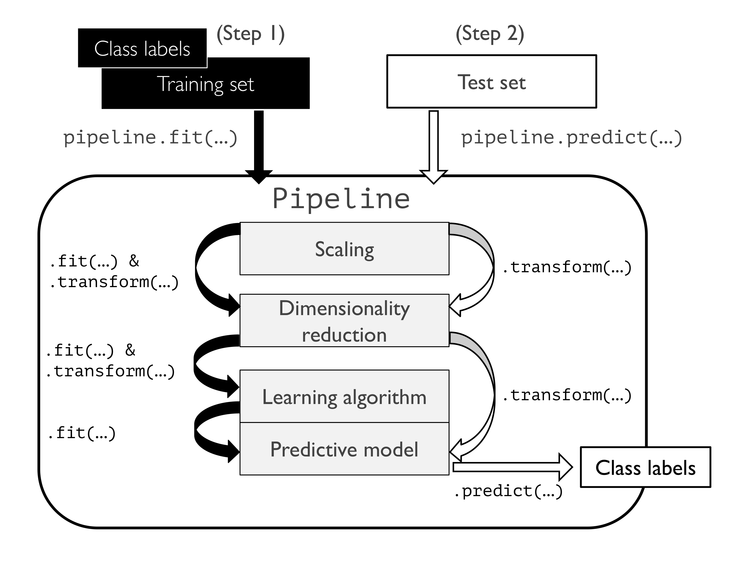
The make_pipeline function takes an arbitrary number of scikit-learn transformers (objects that support the fit and transform methods as input), followed by a scikit- learn estimator that implements the fit and predict methods.

pipline 中可以包含任意个transformer，这个transformer要有fit 和 transform function。pipline的最后是estimator，其要有fit 和 predict function。

If we call the fit method of Pipeline, the data will be passed down a series of transformers via fit and transform calls on these intermediate steps until it arrives at the estimator object (the final element in a pipeline). The estimator will then be fitted to the transformed training data

If we feed a dataset to the predict call of a Pipeline object instance, the data will pass through the intermediate steps via transform calls. In the final step, the estimator object will then return a prediction on the transformed data.

如果我们使用pipline.fit那么pipline中的transformer就会运行fit_transform 的method和estimator的fit method。如果使用pipline.predict，则pipline中的transformer就会运行transform method，estimator 运行predict method。

Using k-fold cross-validation to assess model performance

我们需要把数据进行分割，例如分成train，test dataset。这样的问题是如果我们需要使用 train dataset 来训练模型， test dataset 来评估不同的模型的好坏。如果我们使用test dataset 一次次的用于模型的选择，那么也是变相的使用test dataset 来训练模型。

However, if we reuse the same test dataset over and over again during model selection, it will become part of our training data and thus the model will be more likely to overfit.

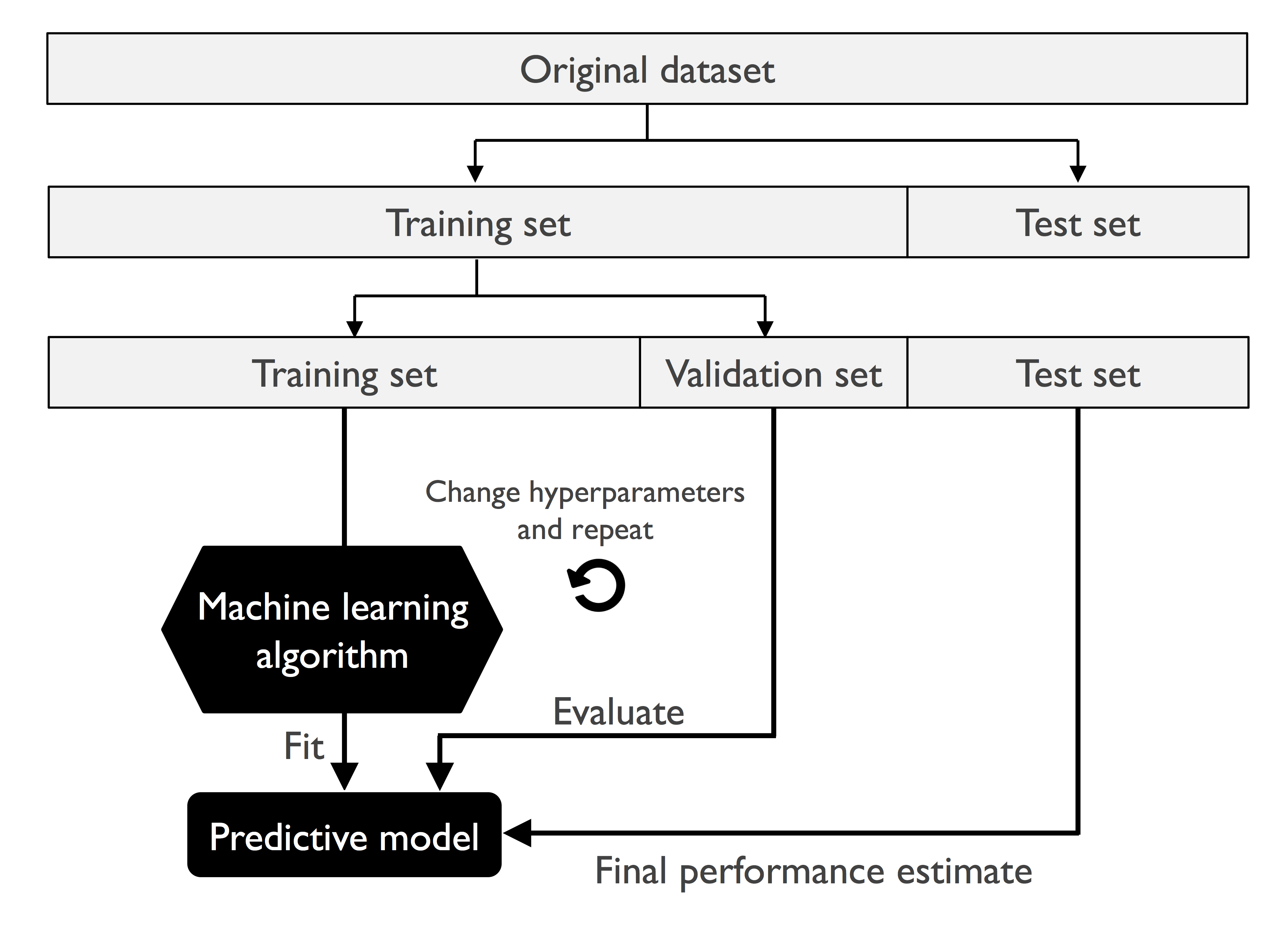
更好的方法是把dataset 分割成：train,validation, test dataset.

A better way of using the holdout method for model selection is to separate the data into three parts: a training dataset, a validation dataset, and a test dataset.

K-fold cross-validation

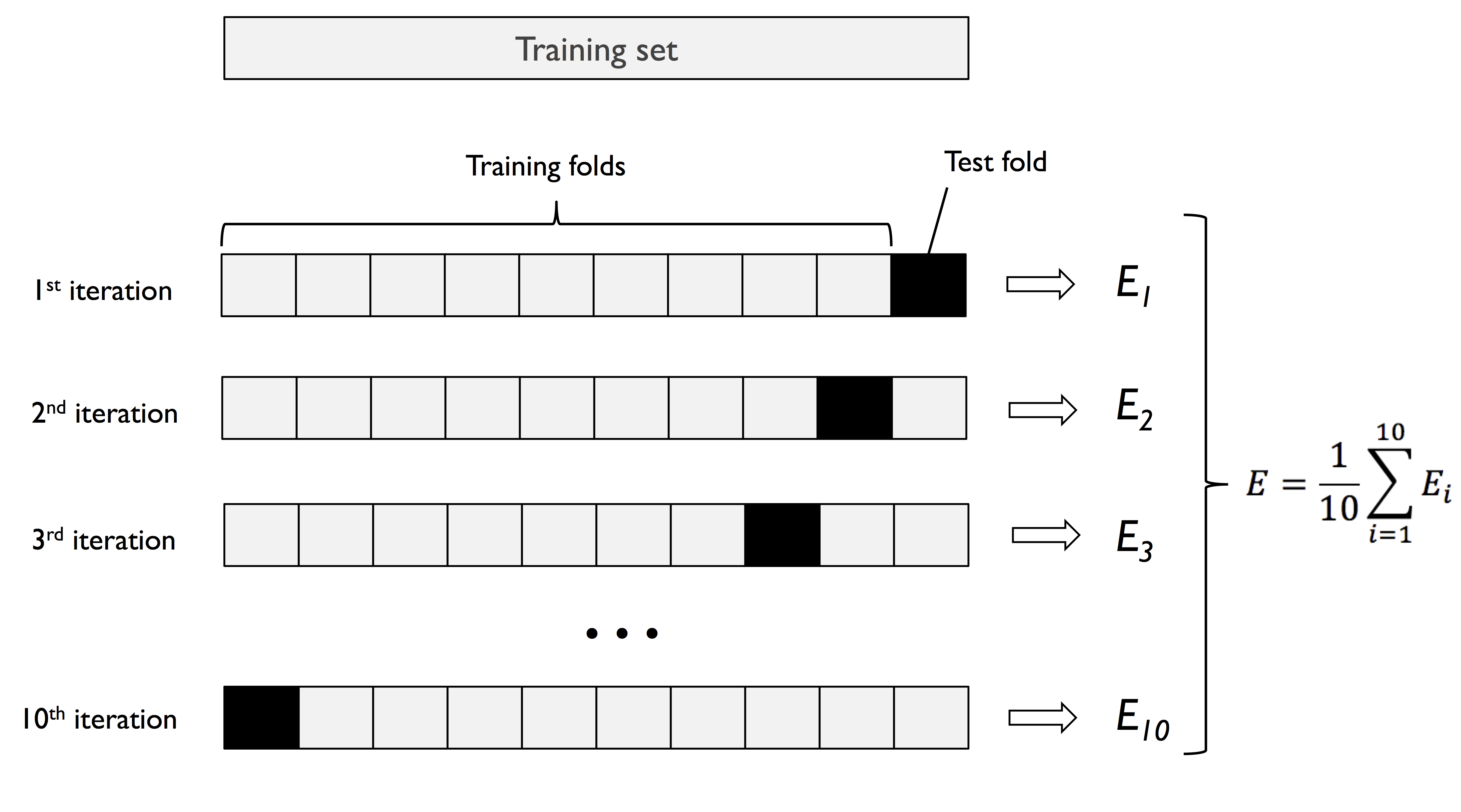
另一种更好的分割数据并进行训练和选择，最后再进行验证的方法是k-fold cross-validation.

采取不放回的抽样方法，把training dataset 分割成为k份。然后使用k-1份的数据用于训练模型，剩下的一份用于model selection 评估模型的performance。这种过程重复k次，这样我们可以得到k个训练好的模型和performance estimates。然后再求均值就可以得到这个模型的好坏。

通过performance estimates 的均值，我们选择出了model并得到了这个模型的最优参数。下一步，再使用整个training dataset 来训练选择出来的模型。 最后使用test dataset来对模型做最后的评估。

Since k-fold cross-validation is a resampling technique without replacement, the advantage of this approach is that each example will be used for training and validation (as part of a test fold) exactly once, which yields a lower-variance estimate of the model performance than the holdout method.

一般k值选择10。如果是非常少的数据，那么k值会增大。如果数据很多，k也可以选择5。

k值增大，那么model training的数据的相似性会变大，因此导致模型的variance会变大(发生 overfitting)。

对于k-fold cross vallidation方法的改进是stratified k-fold cross-validation, which can yield better bias and variance estimates, especially in cases of unequal class proportions。

In stratified cross- validation, the class label proportions are preserved in each fold to ensure that each fold is representative of the class proportions in the training dataset。

使用sklearn 自带的Stratified KFold function.

import numpy as np
from sklearn.model_selection import StratifiedKFold

kfold = StratifiedKFold(n_splits=10).split(X_train,y_train)

scores = []
for k,(train,test) in enumerate(kfold):
    pipe_lr.fit(X_train[train],y_train[train])
    score = pipe_lr.score(X_train[test],y_train[test])
    scores.append(score)
    print('Flod: %2d, Class dist.: %s, Acc: %.3f'%(k+1,
        np.bincount(y_train[train]), score))

StratifiedKFold(n_splits=10).split 把数据分割成10份， 返回的是indinces。在使用split分割时是根据y值进行stratify。

除了上述一种方法，我们还可以直接使用cross_val_score 直接评估model estimates。

from sklearn.model_selection import cross_val_score

scores = cross_val_score(estimator=pipe_lr,
                        X=X_train,
                        y= y_train,
                        cv=10,
                        n_jobs=1)

使用cross_val_score 的方法好处时可以多线程处理。当n_jobs=-1，使用全部的CUP同时进行处理。

Debugging algorithms with learning and validation curves

模型常见的两种问题时high bias and high variance.如下所示

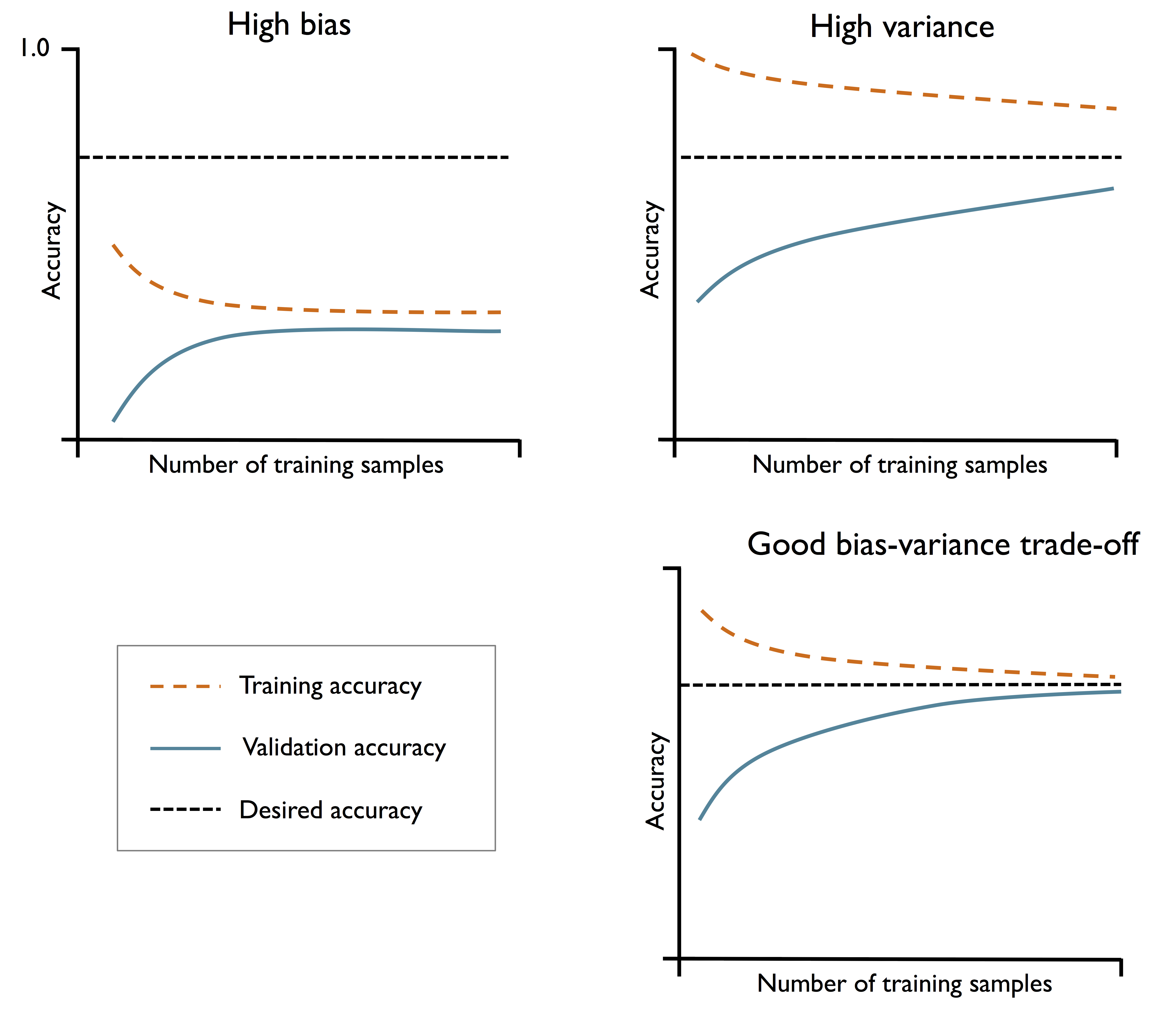
如果时underfitting,采取的策略是：

• 增加模型的参数，让模型变得复杂。
• 收集更多的features，或者构建新的features
• 通过降低regularization的程度，如SVM或者logic regression

如果是overfitting，采取的策略是：

• 收集更多的数据samples
• 减少模型的复杂度
• 增加regularization 的程度
• 减少feature 的维度，降维

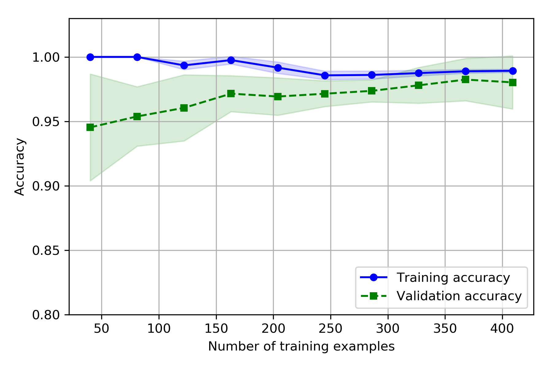
如果增加training samples 用于训练则可能会导致overfitting，因此多少的train samples 比较合适呢？可以使用skealrn 中的learning_curve function.

import matplotlib.pyplot as plt
from sklearn.model_selection import learning_curve
pipe_lr = make_pipeline(StandardScaler(),
                       LogisticRegression(penalty='l2',
                                         random_state=1,
                                         solver='lbfgs',
                                         max_iter=10000))

train_sizes,train_scores, test_scores = \
learning_curve(estimator=pipe_lr,
              X=X_train,
              y= y_train,
              train_sizes=np.linspace(0.1,1.0,10),
              cv=10, # 将xfenge成几分，如果是整数则是按照stratified k-fold方法进行分割
              n_jobs=1) # n_jobs=-1 使用全部的CPU进行计算

train_mean = np.mean(train_scores, axis=1)
train_std = np.std(train_scores,axis=1)

test_mean = np.mean(test_scores,axis=1)
test_std = np.std(test_scores, axis=1)

plt.plot(train_sizes,train_mean,color='blue',
        marker='o',
        markersize=5, label='Training accuracy')
plt.fill_between(train_sizes,
                train_mean+train_std,
                train_mean-train_std,
                alpha=0.15,
                color='blue')
plt.plot(train_sizes,test_mean,color='green', linestyle='--',
        marker='s',markersize=5,
        label='Validation accuracy')
plt.fill_between(train_sizes,
                 test_mean+test_std,
                 test_mean-test_std,
                 alpha = 0.15,
                 color='green'
                )
plt.grid()
plt.xlabel('Number of training examples')
plt.ylabel('Accuracy')
plt.legend(loc='lower right')
plt.ylim([0.8,1.03])
plt.show()

learning_curve : Determines cross-validated training and test scores for different training set sizes.根据training size的不同返回train score and test score.

np.linspace 的用法参考python 只是点

plt.fill_between : 是在train_mean+train_std,train_mean-train_std之间填充，x轴为train_sizes.详细内容可参考matplotlib

plt.grid() : 在图中画出格子线

Addressing over- and underfitting with validation curves

validation curve 与learning curve 很相似。不同之处是learning curve是根据train size的大小求得train score 和test score。而validation curve 则是可以人为地调控模型内的参数，这样就可以在模型发生over - and underfitting时对模型进行调控，看哪一个参数更合适。

在sklearn中使用validation_curve

from sklearn.model_selection import validation_curve
param_range = [0.001,0.01, 0.1, 1.0, 10.0, 100.0]
# param_range = [10, 100,1000]
train_scores, test_scores = validation_curve(estimator=pipe_lr,
                                            X=X_train,
                                            y= y_train,
                                            param_name='logisticregression__C',
                                            param_range=param_range,
                                            cv=10)

train_mean= np.mean(train_scores,axis=1)
train_std = np.std(train_scores,axis=1)
test_mean = np.mean(test_scores,axis=1)
test_std = np.std(test_scores, axis=1)

plt.plot(param_range,train_mean,
        color='blue',marker='o',
        markersize=5,label='Training accuracy')
plt.fill_between(param_range,train_mean+train_std,
                train_mean-train_std,
                alpha=0.15,
                color='blue')
plt.plot(param_range,test_mean,
        color='green',linestyle='--',
        marker='s',markersize=5,
        label='Validation accuracy')
plt.fill_between(param_range,test_mean+test_std,
                test_mean-test_std,alpha=0.15,
                color='green')
plt.grid()
plt.xscale('log')
plt.legend(loc='lower right')
plt.xlabel('Parameter C')
plt.ylabel('Accuracy')
plt.ylim([0.8,1.0])
plt.show()

有以上代码可以看出validation curve需要确定对哪个parameter进行优化(param_name)，以及优化的范围是多少(param_range)。

这里需要注意的是param_name中引用的参数是pipline中LogisticRegression中的参数，由于在pipline中会把名称都变为小写，因此使用logisticregression__C，C为LR中的参数，中间的连接使用双下划线。

Fine-tuning machine learning models via grid search

Learning curve 是对train sizes进行优化，validation curve是对某一参数进行优化。如果相对多个参数进行优化，那么我们则需要grid search。

在机器学习中我们有两类参数需要优化：

• those that are learned from the training data, for example, the weights in logistic regression。需要通过training data训练模型的weights。
• the parameters of a learning algorithm that are optimized separately。the regularization parameter in logistic regression or the depth parameter of a decision tree. 模型本身需要认为设定的参数，例如L1 或者L2 regularization 的程度，Decision tree 的深度，random forest 中树的数目。

The grid search approach is quite simple: it’s a brute-force exhaustive search paradigm where we specify a list of values for different hyperparameters, and the computer evaluates the model performance for each combination to obtain the optimal combination of values from this set。

直接使用sklearn 中的GridSearchCV

from sklearn.model_selection import GridSearchCV
from sklearn.svm import SVC

pipe_svc = make_pipeline(StandardScaler(),
                        SVC(random_state=1))

param_range = [0.0001, 0.001, 0.01, 0.1,
              1.0, 10.0, 100.0, 1000.0]

param_grid = [
    {
        'svc__C':param_range, # 使用pipline中的引用规则
        'svc__kernel':['linear']
    },
    {
        'svc__C':param_range,
        'svc__gamma':param_range,
        'svc__kernel':['rbf']
    }
]

gs = GridSearchCV(estimator=pipe_svc,
                 param_grid=param_grid,
                 scoring='accuracy',
                 cv=10,
                 refit=True,
                 n_jobs=-1)


gs = gs.fit(X_train,y_train)

print(gs.best_score_)

print(gs.best_params_)

clf = gs.best_estimator_

gs.best_score_ : 获得模型最高的值； gs.best_params_ : 获得模型最高的值的参数 ; gs.best_estimator_ : 获得最好的模型.

由于我们在GridSearchCV中设定了refit=True,那么模型在找到最高的score的参数时，会使用全部的X_train，y_train再训练这个模型一次。相当于如下代码：

clf = gs.best_estimator_ # 得到含有最佳参数的模型，如果refit=True，那么下面那一步其实时没有必要的。
 
clf.fit(X_train,y_train)

Grid search 是对全部可能性的参数组合进行尝试，这会带来很大的运算量。另一种可替代的方法是RandomizedSearchCV。这种方法只是从参数中sample 一些参数进行随机组合，然后判定模型的优劣。这种方法适用于参数是连续性分布且非常多的参数的情况。

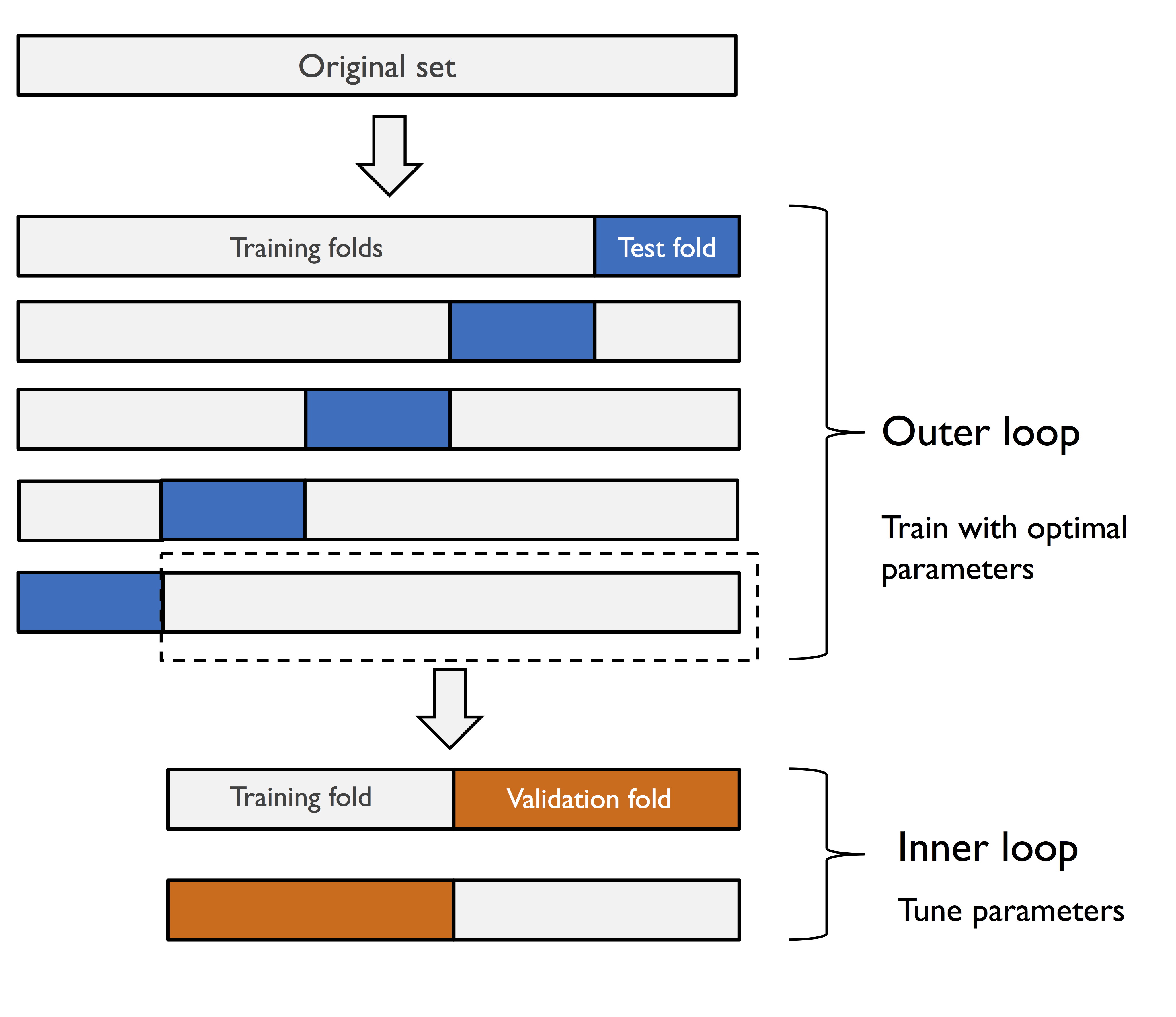
nested cross-validation

如果我们既想调节模型的参数，同时也想在不同的模型中选择合适的模型。那么我们可以把GridSearchCV和cross_val_score结合在一起。其基本流程如下：

1. 外层循环是把数据进行k-fold cross-validation,把数据分割成train_set and test set。
2. 内部还有一个循环那就是对当模型进行调节参数。此时一般是把train data set分割成两份，一份用于train model，一份用于validation model。然后找到在当前数据下最优参数的模型。
3. 使用上一步中的最优参数模型对test set进行评估分数，得到k个score。一般第一步是k=5,第三步cv=2；

In nested cross-validation, we have an outer k-fold cross-validation loop to split the data into training and test folds, and an inner loop is used to select the model using k-fold cross-validation on the training fold. After model selection, the test fold is then used to evaluate the model performance. The following figure explains the concept of nested cross-validation with only five outer and two inner folds, which can be useful for large datasets where computational performance is important; this particular type of nested cross-validation is also known as 5x2 cross-validation:

gs = GridSearchCV(estimator=pipe_svc,
                 param_grid=param_grid,
                 scoring='accuracy', # 使用accuracy作为选择模型的依据
                 cv=2) # 内层循环把数据分割成2份，然后选择出最优参数的模型

scores = cross_val_score(gs,X_train,y_train,
                        scoring='accuracy',cv=5) # 这是外层循环，把original dataset 分割成为5份。对test set 求值时使用accuracy。

np.mean(scores),np.std(scores)
# output : (0.9736263736263737, 0.014906219743132467)

from sklearn.tree import DecisionTreeClassifier
gs = GridSearchCV(estimator=DecisionTreeClassifier(random_state=0),
                 param_grid=[{'max_depth':[1,2,3,4,5,6,7,None]}],
                 scoring='accuracy',
                 cv=2)

scores = cross_val_score(gs,X_train,y_train,
                        scoring='accuracy',cv=5)

np.mean(scores),np.std(scores)
# output:(0.9340659340659341, 0.015540808377726326)

从以上代码的运行结果中可以看出SVM(97.4 percent) 要比decision tree(93.4 percent) 的结果要好。因此对当前数据集来说选择SVM会更好。

GridSearchCV 中的accuracy 是用于比较哪个参数组合能得到更好的模型；而cross_val_score 中的scoring则可认为是通过fit得出的test set 的结果。

Looking at different performance evaluation metrics

仅仅使用accuracy作为评估模型好坏是不够的。因为有时数据是不均衡的。整体来说对于模型的评估需要用到confusion matrix，A confusion matrix is simply a square matrix that reports the counts of the true positive (TP), true negative (TN), false positive (FP), and false negative (FN) predictions of a classifier。如下：

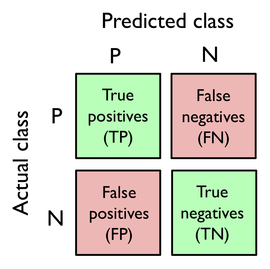
我们的目的是让TP和TN尽可能的大，而FN，FP尽可能的小。

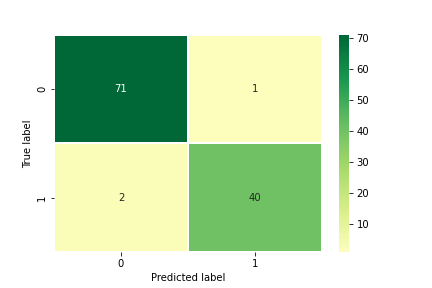
我们下面使用sklearn求出confusion matrix，并用seaborn中的heatmap 画出图来

from sklearn.metrics import confusion_matrix
pipe_svc.fit(X_train,y_train)

y_pred = pipe_svc.predict(X_test)
confmat = confusion_matrix(y_true=y_test,y_pred=y_pred)

import seaborn as sns

sns.heatmap(confmat,
            center=0, 
            annot = True,
            cmap='RdYlGn', 
            linewidths=0.2)
plt.xlabel('Predicted label')
plt.ylabel('True label')
plt.show()

在heatmap中通过使用xticklabels, yticklabels来设置x轴和y轴的刻度名称。使用plt.xlabel and plt.ylabel来设置图中x轴和轴的标签。具体的使用用法可以参考官方文档。

precision and recall of a classification model

Both the prediction error (ERR) and accuracy (ACC) provide general information about how many examples are misclassified. 如果数据有偏差，那么即使得到很高的ACC也没有太大的意义。例如99%的case 是negative，1%的case是positive。

The true positive rate (TPR) and false positive rate (FPR) are performance metrics that are especially useful for imbalanced class problems:

例如在肿瘤诊断中，我们更关注恶性肿瘤是否能被识别出来，因为不想耽误治疗。因此如果在数据中患有肿瘤的标签为1(positive),那么我们希望TPR越高越好。

The performance metrics precision (PRE) and recall (REC) are related to those TP and TN rates, and in fact, REC is synonymous with TPR:

precision(精度)是指在模型判定为true positive的cases中有多少是真正的true positive cases。

recall(召回率)是指在ture positive 的cases中模型判定了多少cases为ture positive。

如果我们想平衡PRE and REC，我们可以使用F1 score。

ACC, recall and f1 score 在sklearn中有function 可用

from sklearn.metrics import precision_score
from sklearn.metrics import recall_score,f1_score

precision_score(y_true=y_test,y_pred=y_pred)

recall_score(y_true=y_test,y_pred=y_pred)

f1_score(y_true=y_test,y_pred=y_pred)

在sklearn中默认positive label为1，我们可以使用sklearn中的make_scorer 人为设定positive label的的标签。

from sklearn.metrics import make_scorer, f1_score

c_gamma_range = [0.01,0.1,1.0, 10.0]
param_grid = [
    {'svc__C':c_gamma_range,
    'svc__kernel':['linear']
    },
    {
        'svc__C':c_gamma_range,
        'svc__gamma':c_gamma_range,
        'svc__kernel':['rbf']
    }
]

scorer = make_scorer(f1_score,pos_label=0) # 更换positive labe

gs = GridSearchCV(estimator=pipe_svc,
                 param_grid=param_grid,
                 scoring=scorer, # 使用更换后的label，以及评判标准score。
                 cv=10)
gs = gs.fit(X_train, y_train)

gs.best_score_

gs.best_params_

Receiver operating characteristic (ROC)

ROC是根据FPR和TPR来评估分类模型的performace。如果是一个二分类的问题，那么ROC如果是一条对角线，那么认为此时的模型是random gussing。因此ROC在对角线上越靠上越好。

使用sklearn 和 matplotlib画ROC

from sklearn.metrics import roc_curve, auc

from scipy import interp # 通过插值法填补缺失值

pipe_lr = make_pipeline(StandardScaler(),
                       PCA(n_components=2),
                        LogisticRegression(
                            penalty='l2',
                            random_state=1,
                            solver='lbfgs',
                            C=100.0))

X_train2 = X_train[:, [4,14]]

cv = list(StratifiedKFold(n_splits=3,
                         random_state=1).split(X_train,
                                              y_train))

mean_tpr = 0.0
mean_fpr = np.linspace(0,1,100) # x轴的间隔点
all_tpr = []

for i, (train,test) in enumerate(cv):
    probas = pipe_lr.fit(
        X_train2[train],
        y_train[train]).predict_proba(X_train2[test]) # 概率值，每个class都有一个概率值，shape is [n_samples,2]
    
    fpr, tpr, thresholds = roc_curve(y_train[test],
                                    probas[:,1], # 第二列表示使用positive label的score
                                    pos_label=1)
    
    mean_tpr += interp(mean_fpr, fpr,tpr) # 为了划线多求一些点
    mean_tpr[0] = 0.0
    roc_auc = auc(fpr, tpr)
    plt.plot(fpr,
            tpr,
             label = 'ROC fold %d (area=%0.2f)'%
             (i+1, roc_auc)
            )

plt.plot([0,1],
        [0,1],
        linestyle='--',
        color=(0.6, 0.6,0.6),
        label='Random guessing')

mean_tpr /= len(cv)
mean_tpr[-1] = 1.0
mean_auc = auc(mean_fpr,mean_tpr)
plt.plot(mean_fpr,mean_tpr, 'k--',
        label='Mean ROC (area= %0.2f)'% mean_auc,lw=2)

plt.plot([0,0,1],
        [0,1,1],
         linestyle=':',
         color = 'black',
         label = 'Perfect performance'
        )

plt.xlim([-0.05,1.05])
plt.ylim([-0.05,1.05])


plt.xlabel('False positive rate')
plt.ylabel('True positive rate')
plt.legend(loc='lower right')
plt.show()

Scoring metrics for multiclass classification

以上的模型评判标准都是以二分类模型为准。但是sklearn为了使用以上的标准，通过one-vs.-all(OvA)的方法计算模型的macro 和 micro标准。即通过判断一个模型能否区分class_a and class_else。

micro 的精度是所有的class能正确分成positive 的与所有模型预测称positive的比例。例如有4个classes，class 0 的label 为1 class other(class 1,2,3) 的label 为0.以此类推。

macro 的计算是把所有class的micro PRE求一个平均值

此时

从上面的公式中可以看出，如果我们看重model对每一个class的分类表现，那么我们可以选择micro-averaging，因此每个model对每个class的表现都体现在了分子和分母上； 如果看重模型的整体结果(而不是每个class的结果)，那么macro-averaing更合适，因为它更看重most frequent class labels.

Micro-averaging is useful if we want to weight each instance or prediction equally, whereas macro-averaging weights all classes equally to evaluate the overall performance of a classifier with regard to the most frequent class labels.

If we are using binary performance metrics to evaluate multiclass classification models in scikit-learn, a normalized or weighted variant of the macro-average is used by default. The weighted macro-average is calculated by weighting the score of each class label by the number of true instances when calculating the average. The weighted macro-average is useful if we are dealing with class imbalances, that is, different numbers of instances for each label.

如果dataset中每个class的data 是不平衡的，那么需要根据每个class 的positiv case的数量在每个class的PRE前面添加weights。在sklearn中对于多分类的问题，sklearn会默认为使用weighted macro-average 作为评判标准。

Dealing with class imbalance

对于不平衡的数据有以下方法：

1. One way to deal with imbalanced class proportions during model fitting is to assign a larger penalty to wrong predictions on the minority class. 对于数目较少的class，在fitting的过程中如果出现错误分配，那么会增加一个更大的惩罚。起到一个矫正的作用。
2. upsampling the minority class, downsampling the majority class, and the generation of synthetic training examples. 另一种方法是扩大少数class的样本，减少多数样本class的样本数目，最后是合成新的数据。

对于upsample 可以使用sklearn中的resample

from sklearn.utils import resample

X_imb = np.vstack((X[y==0], X[y==1][:40]))# 生成不平衡的dataset
y_imb = np.hstack((y[y==0], y[y==1][:40]))

X_imb[y_imb==1].shape

X_upsampled,y_upsampled = resample( 
    X_imb[y_imb == 1],
    y_imb[y_imb == 1],
    replace = True,
    n_samples = X_imb[y_imb == 0].shape[0],
    random_state = 123
    )

X_upsampled.shape[0]

X_bal = np.vstack((X[y==0],X_upsampled))
y_bal = np.hstack((y[y==0], y_upsampled))

np.bincount(y_bal)
# array([357, 357])

resample function 中前两个参数是要进行resample的样本，replace=True，说明是有放回的取样，n_samples = number 是要最终生成的样本数目。具体的参数内容可查看官方文档。

Combining Different Models for Ensemble Learning

这一章主要讲以下内容：

• Make predictions based on majority voting
• Use bagging to reduce overfitting by drawing random combinations of the training dataset with repetition
• Apply boosting to build powerful models from weak learners that learn from their mistakes

Ensemble method 就是把多个classifier整合在一起，然后输出的结果要比单个classifier的结果要好。

The goal of ensemble methods is to combine different classifiers into a meta- classifier that has better generalization performance than each individual classifier alone.

Majority vote

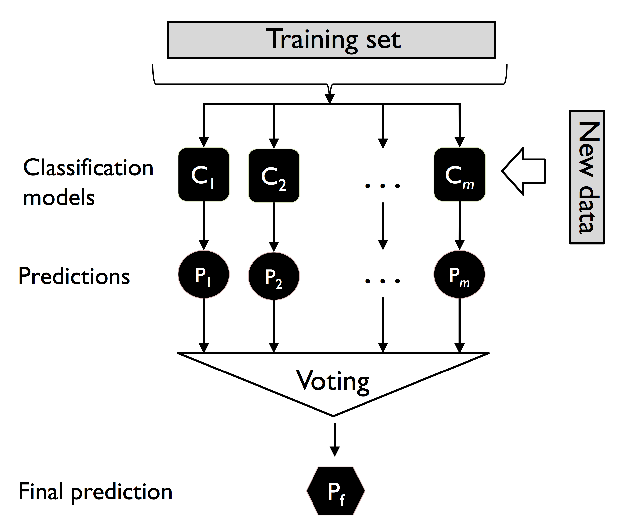
majority vote是使用同一个dataset训练不同的classifiers，然后对所有classifier的预测结果中，看哪个预测结果出现的频次最多就认为这个结果是最终结果。

为社么ensemble method 会比单个classifier的结果好

可以通过对二分类classifier的ensemble method举例说明。

当每个classifier都有相同的error rate(e) 时, ensembel 的error rate可以使用二项式分布来计算ensemble method 的错误率是比单个classifier的错误率要低。

例如有11个二分类classifier，每个classifier的错误率为0.25，那么计算ensemble的错误率如下：

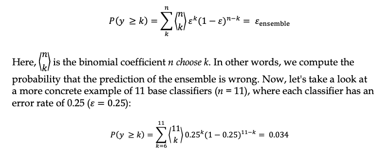
0.034 要远比0.25的错误率要小很多。

Majority vote classifier

如果需要给每个classifier都加上一个权重(weights),那么每个结果都应乘以权重以后再进行判断。如下：

在书本中有从头创建MajorityClassifier class的代码和应用。现在sklearn中也已经创建了相应的function sklearn.ensemble.VotingClassifier

Bagging

Bagging 就是有放回地取样。在上面的Majority classifier中每一个classifier都使用相同的datase来进行trian。使用Bagging就可以使用不同的dataset来进行training。

In fact, random forests are a special case of bagging where we also use random feature subsets when fitting the individual decision trees.

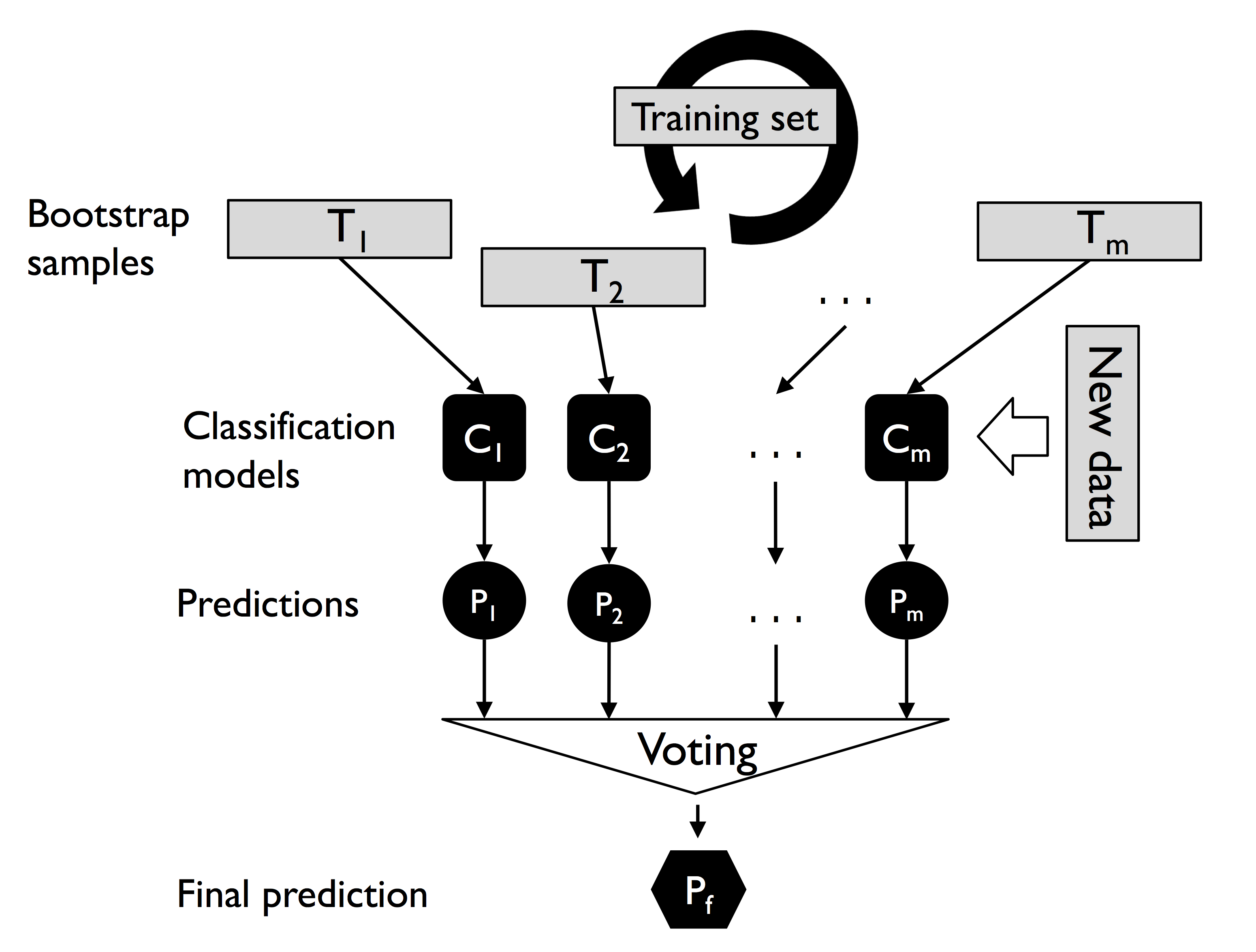
在sklearn中已有sklearn.ensemble.BaggingClassifier可以使用。

from sklearn.ensemble import BaggingClassifier

tree = DecisionTreeClassifier(criterion='entropy',
                             random_state=1,
                             max_depth=None)
bag = BaggingClassifier(base_estimator=tree,
                       n_estimators=500,
                       max_samples=1.0,
                       max_features=1.0,
                       bootstrap=True,
                       bootstrap_features=False,
                       n_jobs=1,
                       random_state=1)

从以上代码中我们可以看出Bagging 使用同一种classifier，只是使用不同的samples来训练同一种classifier，从而得到多个classifiers。这样可以避免hight variance。防止classifer使用整个dataset产生overfitting.

boosting

boosting 含有多个classifiers，每次traing后可以得到错误的datasets，然后再把错误的dataset的weights调大。这样每次training都会调节weights，修改classifier的参数。然后得到训练好后的classifiers。当有新的数据要predict时，就可以使用Majority voting 的策略得到新数据的label。

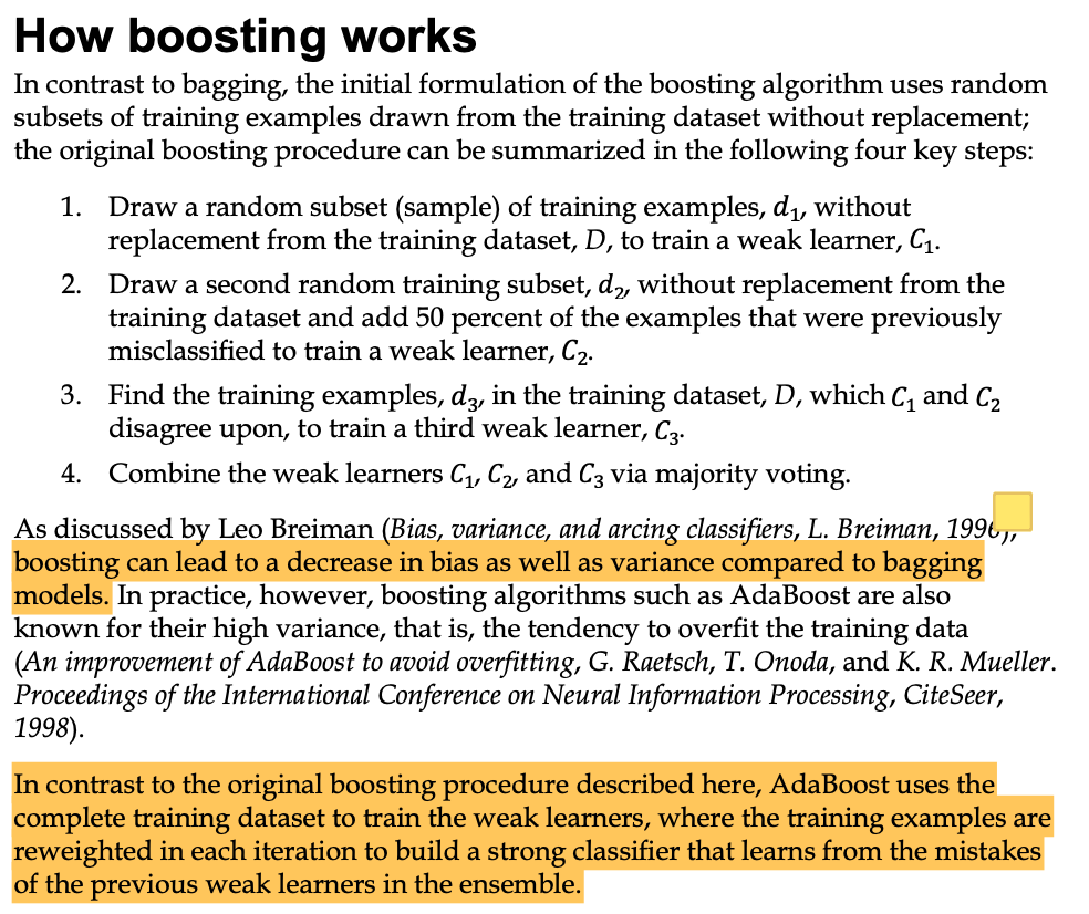
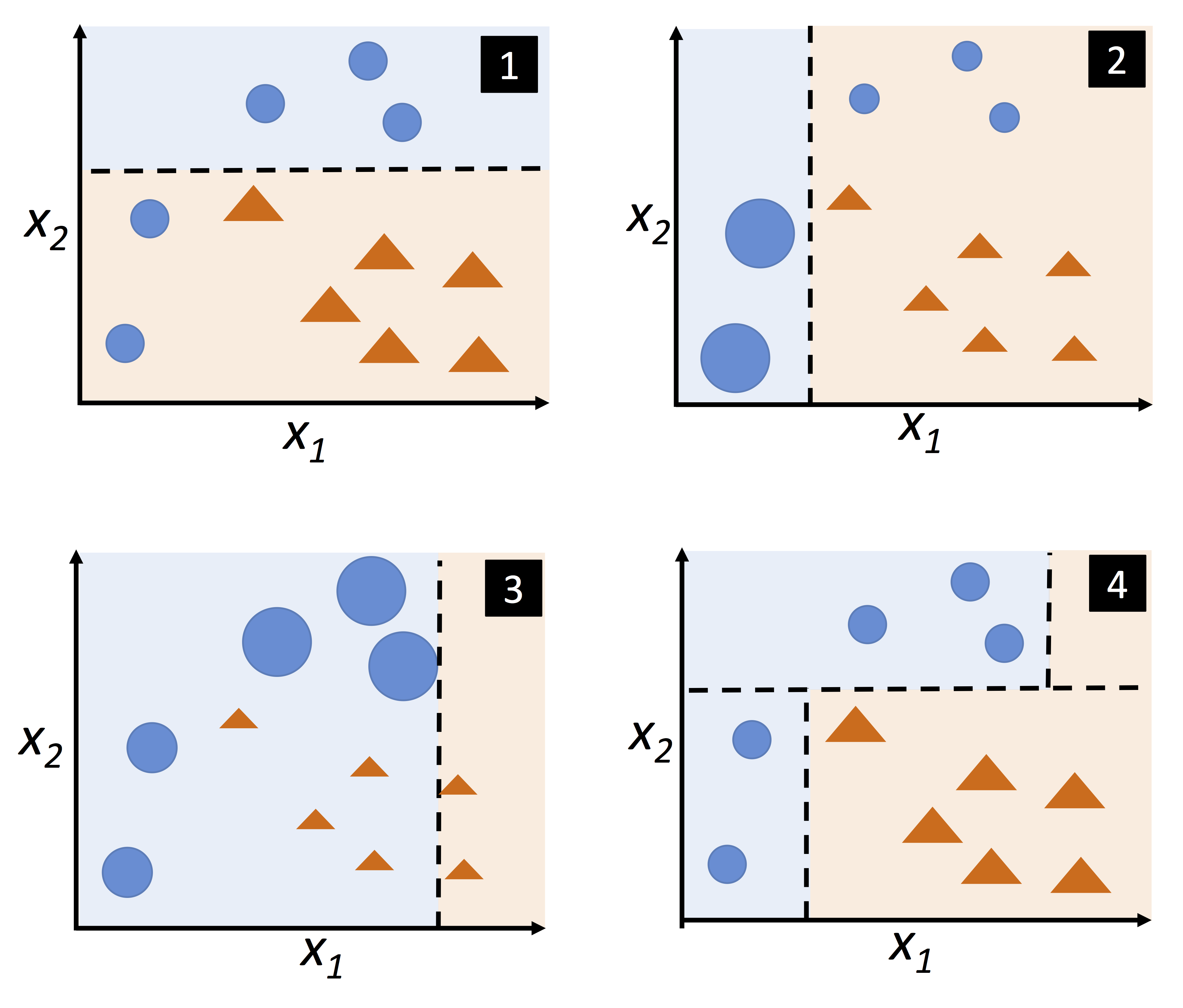
figure 1，2，3是相同的classifiers。2是在1的基础上对samples的weights进行调节后的再训练。3是在2的基础上的再训练。4是majority vote的结果。

sklearn 中已有sklearn.ensemble.AdaBoostClassifier.

from sklearn.ensemble import AdaBoostClassifier

tree = DecisionTreeClassifier(criterion='entropy',
                             random_state=1,
                             max_depth=1)

ada = AdaBoostClassifier(base_estimator=tree,
                        n_estimators=500,
                        learning_rate=0.1,
                        random_state=1)

tree = tree.fit(X_train,y_train)

y_train_pred = tree.predict(X_train)

ada = ada.fit(X_train,y_train)

ada.score(X_train,y_train)

ada.score(X_test,y_test)